2024

Day 2

Notebook: make changes to your module's code and see the effects immediately without needing to manually reload or restart the notebook's kernel.

%load_ext autoreload # enable the autoreload feature in your notebook session.
%autoreload 2 #  sets the auto-reload mode to "2", which means that modules will be automatically re-loaded before executing any code that depends on them.

How to express $10^{n}$: 2.944297e+10 is equivalent to 2.944297*(10**10)

Day 1

Matplotlib

Modify the x-axis with highlighted values (only), instead of listing down all the dates
- In the below example, instead of putting in x-axis all the months, we just highlight data points with marks a year from 1949 to 1962

fig, ax = plt.subplots()

ax.plot(df['Month'], df['Passengers'])
ax.set_xlabel('Date')
ax.set_ylabel('Number of air passengers')

plt.xticks(np.arange(0, 145, 12),   # only provide each 12 months
           np.arange(1949, 1962, 1) # a list of a year corresponding to
)

Pandas

`.loc` vs `.iloc`

loc gets rows (and/or columns) with particular labels.
iloc gets rows (and/or columns) at integer locations.
Example: given the following dataframe that has the index starting from 80 to 84

df = pd.DataFrame(np.arange(25).reshape(5, 5),
                      index=[80, 81, 82, 83, 84],
                      columns=['col_A','col_B','col_C', 'col_D', 'col_E'])

	col_A	col_B	col_C	col_D	col_E
80	0	1	2	3	4
81	5	6	7	8	9
82	10	11	12	13	14
83	15	16	17	18	19
84	20	21	22	23	24

Return the first row of the df with two columns col_A and col_D
- .loc: since the first row in the dataframe corresponding to the index=80, so we need to specify it in the .loc
  - df.loc[80, ["col_A", "col_D"]]
- .iloc: as iloc will be based on the integer location, so the first row in the df is corresponding to the location 0
  - df.iloc[0, [df.columns.get_loc(c) for c in ["col_A", "col_D"]]]

# example of .loc and .iloc to return the first row of the df with two columns A and D
df.loc[80, ["col_A", "col_D"]]
# col_A    0
# col_D    3
df.iloc[0, [df.columns.get_loc(c) for c in ["col_A", "col_D"]]]
# col_A    0
# col_D    3

Select last 2 row in the df → .iloc will have the advantages as it is based on the integer location rather then the labels.

df.iloc[-2:, :]

	col_A	col_B	col_C	col_D	col_E
83	15	16	17	18	19
84	20	21	22	23	24

Select first 3 columns of the row after index=82

df.iloc[df.index.get_loc(82):, :3]

	col_A	col_B	col_C
82	10	11	12
83	15	16	17
84	20	21	22

2023

Day 11

Python

1e-4 is equal to 0.0001 with total 4 zeros
Validate the input string variable, say split belongs to certain options: assert split in ['train', 'test', 'both']
- We can add the handling path if the assertion error paused the program
```
try:
    assert 'value' not in numerical_vars
except AssertionError:
    # do something
```

Pandas

`pd.melt` vs contingency table (`pd.crosstab`)

The melt function in pandas is used to unpivot a DataFrame, meaning that it converts columns of data into rows.
- This is useful when you want to combine the data for plotting
- For example: the melt function has converted the Math and Physics columns into rows, and created two new columns: subject and score.

# Create a sample DataFrame
df = pd.DataFrame({'student_id': [1, 2, 3], 'Math': [4, 5, 6], 'Physics': [7, 8, 9]})

# Melt the DataFrame
df_melted = df.melt(id_vars=['student_id'], value_vars=['Math', 'Physics'], var_name='Ssubject', value_name='score')

# Print the melted DataFrame
print(df_melted)

#    student_id subject  score
# 0       1      Math      4
# 1       2      Math      5
# 2       3      Math      6
# 3       1      Physics   7
# 4       2      Physics   8
# 5       3      Physics   9

# plotting the melted dataframe by subject using hue of seaborn

sns.barplot(df_melted, x='student_id', y='score', hue='subject')

The crosstab function: produces a DataFrame where the rows represent the levels of one factor and the columns represent the levels of another factor.
Usage: to create frequency table for each category in a feature vs another feature
The crosstab function takes the following arguments:
- index: The name of the column to use for the row labels.
- columns: The name of the column to use for the column labels.
- values: The name of the column to use for the cell values. If not specified, the counts of observations are used.
- margins: If True, the DataFrame will include a row and column for the totals.

# Create a sample DataFrame
df = pd.DataFrame({'gender': ['M', 'F', 'M', 'F', 'F'], 'favorite_color': ['blue', 'red', 'green', 'blue', 'purple']})

#     gender favorite_color
# 0      M           blue
# 1      F            red
# 2      M          green
# 3      F           blue
# 4      F         purple
# Create a crosstabulation of gender and favorite color
crosstab = pd.crosstab(df['gender'], # rows
                       df['favorite_color'],  # columns
                       margins=True # True to calculate the total
                       )

# re-name columns "All" to 'row_totals' & 'col_totals'
# note: columns "All" are only avail if margins=True
crosstab.columns = [*crosstab.columns.to_list()[:-1], 'row_totals']
crosstab.index = [*crosstab.index.to_list()[:-1], 'col_totals']
#             blue  green  purple  red  row_totals
# F              1      0       1    1           3
# M              1      1       0    0           2
# col_totals     2      1       1    1           5

Matplotlib

Subplots:

# Annual, weekly and daily seasonality
# ==============================================================================
fig, axs = plt.subplots(2, 2, figsize=(8.5, 5.5), sharex=False, sharey=True)

# Before:
ax1 = axs[0,0]
ax2 = axs[0,1]
# After with axs.ravel()
axs = axs.ravel()
ax1 = axs[0]
#...
ax4 = axs[3]

Conda vs Pip: Package Availability

Pip installs packages from the Python Package Index (PyPI), which hosts a vast array of Python libraries. Almost any Python library can be installed using pip.
conda installs packages from the Anaconda distribution and other channels (conda-forge). While the number of packages available through conda is smaller than pip, conda can install packages for multiple languages and not just Python.
Example: skforecast is not avail in the conda-forge but it is avail in PyPI, so you cannot conda install skforecast, but it can be install via pip install command

Day 10

Pandas

Find the row with the column is equal to value: index_choice = df.index.get_loc(CustomerId=15674932)

`pd.cut` vs `pd.qcut`

	Space between 2 bins	Frequency of Samples in each bin
`pd.cut`	Equal Spacing	Difference
`pd.qcut`	Un-equal Spacing	Same

pd.cut will choose the bins to be evenly spaced according to the values themselves and not the frequency of those values.
- You also can define the bounds for each binning with pd.cut()
- You can use the Fisher-Jenks algorithm to determine the natural bounds and then pass those values into pd.cut()
pd.qcut the bin interval will be chosen so based on the percentiles that you have the same number of records in each bin.

factors = np.random.randn(30)

pd.cut(factors, 5).value_counts() # bin size has equal interval of ~1

# (-2.583, -1.539]    5
# (-1.539, -0.5]      5
# (-0.5, 0.539]       9
# (0.539, 1.578]      9
# (1.578, 2.617]      2

pd.qcut(factors, 5).value_counts() # each bin has equal size of 6

# [-2.578, -0.829]    6
# (-0.829, -0.36]     6
# (-0.36, 0.366]      6
# (0.366, 0.868]      6
# (0.868, 2.617]      6

`.read_csv()` by chunk

If the csv file is large, can consider to read by chunk

df_iter = pd.read_csv(file_path, iterator=True, chunksize=100000)
df = next(df_iter)

Python

`lru_cache` from `functools`

@lru_cache modifies the function it decorates to return the same value that was returned the first time, instead of computing it again, executing the code of the function every time.

@lru_cache
def say_hi(name: str, salutation: str = "Ms."):
    return f"Hello {salutation} {name}"

typing `Annotated`

Annotated in python allows developers to declare the type of a reference and provide additional information related to it.

from typing_extensions import Annotated
# This tells that "name" is of type "str" and that "name[0]" is a capital letter.
name = Annotated[str, "first letter is capital"]

Fast API examples:

from fastapi import Query
def read_items(q: Annotated[str, Query(max_length=50)])

The parameter q is of type str with a maximum length of 50.

Float to Decimal conversion

Convert float directly to Decimal constructor introduces a rounding error.

from decimal import Decimal
x = 0.1234
Decimal(x)
# Decimal('0.12339999999999999580335696691690827719867229461669921875')

Solution: to convert a float to a string before passing it to the constructor.
- You also can round the float before converting it to string

Decimal(str(x))
# Decimal('0.1234')
Decimal(str(round(x,2)))
# Decimal('0.12')

Day 9

`subprocess` module

subprocess.run is a higher-level wrapper around Popen that is intended to be more convenient to use.
- Usage: to run a command and capture its output
subprocess.call
- Usage: to run a command and check the return code, but do not need to capture the output.
subprocess.Popen is a lower-level interface to running subprocesses
- Usage: if you need more control over the process, such as interacting with its input and output streams.
A PIPE is a unidirectional communication channel that connects one process's standard output to another's standard input.

# creates a pipe that connects the output of the `ls` command to the input of the `grep` command,
ls_process = subprocess.Popen(["ls"], stdout=subprocess.PIPE, text=True)

grep_process = subprocess.Popen(["grep", ".ipynb"], stdin=ls_process.stdout, stdout=subprocess.PIPE, text=True)

output, error = grep_process.communicate()

print(f"Ouptut:\n{output}")
print(f"Error : {error}")

# Ouptut:
# google_colab_tutorial.ipynb
# subprocess.ipynb
#
# Error : None
result = subprocess.run(["ls"], stdout=subprocess.PIPE)

print(result.stdout.decode()) # decode() to convert from bytes to strings
# google_colab_tutorial.ipynb
# subprocess.ipynb

`subprocess` vs `os.system`

subprocess.run is generally more flexible than os.system (you can get the stdout, stderr, the "real" status code, better error handling, etc.)
Even the documentation for os.system recommends using subprocess instead.

`sys` module

The kernel knows to execute this script with a python interpreter with the shebang #!/usr/bin/env python
sys.argv[0] return name of the script
sys.argv[1:] return the arguments parsed to the script

#############################
# in the python_script.py   #
#############################
#!/usr/bin/env python
import sys
for arg in reversed(sys.argv[1:]):
    print(arg)

#############################
# in the interactive shell  #
#############################
bash-5.2$ chmod +x python_script.py
bash-5.2$ ./python_script.py a b c
# Running: ./python_script.py
# c
# b
# a

Day 8

bytes("yes", "utf-8") convert string to binary objects:

Matplotlib

Color Map

cmap = plt.get_cmap("viridis")
fig = plt.figure(figsize=(8, 6))
m1 = plt.scatter(X_train, y_train, color=cmap(0.9), s=10)
m2 = plt.scatter(X_test, y_test, color=cmap(0.5), s=10)

Plot 2 charts on the same figure with share x-axis

fig, ax1 = plt.subplots()

ax1.hist(housing["housing_median_age"], bins=50)

ax2 = ax1.twinx()  # key: create a twin axis that shares the same x-axis
color = "blue"
ax2.plot(ages, rbf1, color=color, label="gamma = 0.10")
ax2.tick_params(axis='y', labelcolor=color)
ax2.set_ylabel("Age similarity", color=color) # second y-axis's measurement

plt.show()

Relative import

# example.py
from .abstract import ExampleClass
# if we run this script directly like python src/abc/example.py, we will encounter the issue

Soluton: python -m src.abc.example or call the example.py script outside the src

`subprocess.Popen` to send Linux command

from subprocess import Popen, Pipe

execute = Popen("scp -i /location_in_machine_A/to/private/key -v -P 64022 file_path machineB@ip_address:/path/to/store/inB/".split(), stdout=PIPE, stdin=PIPE, stderr=PIPE)
execute.stdin.write(bytes("yes", "utf-8")) # to send the "yes" command
execute.communicate()[0]

`os.path`

To read the path separator of the env os.path.sep # return '/' if using Linux

List

Copy a list: copied_list = a_list[:]
- Leverage on copy module
```
import copy
copied_list = copy.deepcopy(a_list)
```

Day 7

Conda

Conda is an open source package + environment manager
Conda vs (Miniconda & Anaconda):
- Conda is a package manager & Conda is tightly coupled to two software distributions: Anaconda and Miniconda.
- Anaconda is a full distribution of the central software in the PyData ecosystem, and includes Python itself along with binaries for several hundred third-party open-source projects.
- Miniconda is essentially an installer for an empty conda environment, containing only Conda and its dependencies, so that you can install what you need from scratch.
Recommended conda installation in PC: Miniconda
Miniconda and Miniforge:
- Miniforge-installed conda is the same as Miniconda-installed conda, except that it uses the conda-forge channel (and only the conda-forge channel) as the default channel.
- Miniconda-installed conda is the Anaconda (company) driven minimalistic conda installer, where pacakages installed from the anaconda channels
Conda channel: A channel is the location where packages are stored remotely.
- Example of channels: Anaconda channel, conda-forge, Apple
- Install TensorFlow dependencies from Apple Conda channel: conda install -c apple tensorflow-deps
Understanding environment.yml in conda create --prefix ./venv python=3.8 --file environment.yml
- tensorflow-deps will need to be installed by conda via apple channel
- scikit-learn will be installed by conda via conda-forge channel
- tensorflow-macos will need pip install via PyPI

name: tensorflow
channels:
  - apple
  - conda-forge
dependencies:
  - tensorflow-deps
  - scikit-learn
  - pip:
      - tensorflow-macos
      - tensorflow-metal

Conda env creation:

# create env
conda create --prefix ./venv python=3.8 --file requirements.txt
conda activate ./venv
conda deactivate

# install package from requirements.txt
conda install --file requirements.txt
# export to requirements.txt so that can install via pip in virtualenv/venv environment

pip list --format=freeze > requirements.txt

`conda create --file requirements.txt` vs `conda env create --file environment.yml`

conda create --file expects a requirements.txt, not an environment.yml, each line in the given file is treated as a package-reference
conda env create to create an environment from a given environment.yml
- Command: conda env create --name tensorflow --file environment.yml

Other common conda commands

conda env list to list down conda envs
du -h -s $(conda info --base)/envs/* list down the size of each env
conda config --show channels to show available channels in the config

Day 6

Number: 1000000 can be written as 1_000_000 for the ease of visualisation
```
state['Population'] / 1_000_000
```

Matplotlib

Plot horizontal line: {plt, ax}.axhline(y=0.5, color='r', linestyle='-')

Numpy

Stacking columns/rows
- np.column_stack & np.row_stack
- np.hstack & np.vstack

a = np.array((1,2,3))
b = np.array((2,3,4))
# column stack
np.column_stack((a,b))
# array([[1, 2],
#       [2, 3],
#       [3, 4]])

# row_stack or vstack
np.row_stack((a,b))
np.vstack((a,b))
# array([[1, 2, 3],
#        [2, 3, 4]])

# hstack
np.hstack((a,b))
# array([1, 2, 3, 2, 3, 4])

Holidays package

Pandas's holiday package: pandas.tseries.holiday
holidays package

Code Refactor

Instead of if '.yml' in file_path or '.yaml' in file_path we can do as follows:
- Solution: if any(ext in file_path for ext in ['.yml', '.yaml']

Day 5

Seaborn

To get color palatte color_pal = sns.color_palette()

Histogram (Displot)

Since the sns.displot is deprecated, so we will use sns.histplot as follow to plot the histogram + kde distribution by specifying kde=True
Also can set_xlim() to the zone that containing the data in case the distribution is skewed

sns.histplot(df['col_name'], kde=True, bins=50).set_xlim(0,8);

Pairplot

Pairplot is to use scatterplot() for each pairing of the variables and histplot() for the marginal plots along the diagonal
Customise with x_var and y_var and hue

sns.pairplot(df.dropna(),
             hue='hour',
             x_vars=['hour','dayofweek',
                     'year','weekofyear'],
             y_vars='PJME_MW',
             height=5,
             plot_kws={'alpha':0.15, 'linewidth':1.5}
            )
plt.suptitle('Power Use MW by Hour, Day of Week, Year and Week of Year')
plt.show()

Python

yield keyword is used in the context of defining generator functions.
- When a generator function is called, it doesn't execute the function immediately.
- Instead, it returns a generator object that can be used to control the execution of the function.
- The code inside the generator function is executed only when an item is requested from the generator using the next() function or a for loop.

def simple_generator():
    yield 1
    yield 2
    yield 3

# Create a generator object
gen = simple_generator()

# using next() to access the code inside
print(next(gen)) # 1
print(next(gen)) # 2
print(next(gen)) # 3
print(next(gen)) # StopIteration raised

# using for-loop to iterate through the generator
for value in simple_generator():
    print(value)

Pandas

Select columns based on Dtype

Numerical columns: num_cols = df.select_dtypes(include=np.number).columns.tolist()
Categorical columns: cat_cols = df.select_dtypes(exclude=np.number).columns.tolist()

Time-series

Convert the datetime index to a datetime col: df['date'] = df.index.date
Slicing using 1 date by including 23:59:59

end_train = '1980-01-01 23:59:59'
# including 23:59:59 means
data_train = df.loc[:end_train] # ends at 1980-01-01
data_test  = df.loc[end_train:] # start at 1980-01-02

`df.query`

Can set multiple condition: df.query("make == 'bmw' and model == '1_series')
Can query using a list

holiday_list = ['2021-01-01', '2022-09-02']
df.query('datetime_col in @holiday_list')

Check & Remove Duplicates

df.duplicated() to check if there are any row duplicate. This will return True for the 2nd occurence of the duplicate
- df.duplicated(subset=['col_A','col_B','col_C']) in case there is no entire row duplciate, we can check duplicates for only subsets of columns
df.query("make == 'bmw' and model == '1_series' and year == 2013 and price == 31500") using query to identify & view the duplicated rows
Remove the duplicates
- .reset_index(drop=True) to reset the index after dropping the duplicates
- .copy() to make the deep copy of the dataframe

df = df.loc[~df.duplicated(subset=['Coaster_Name','Location','Opening_Date'])] \
    .reset_index(drop=True).copy()

Matplotlib

You can set matplotlib object to ax variable
- You also can continue to plot on the same graph with ax variable

# case 1: get ax from the plot via pandas dataframe
ax = df['year'].value_counts() \
    .head(10) \
    .plot(kind='bar', title='Top 10 Years Coasters Introduced')

# case 1.1: also can continue to plot on the same graph with ax variable
df.query('year < 2023').plot(style='.', ax=ax)

ax.set_xlabel('year')
ax.set_ylabel('count')

# case 2: get ax from the plot via seaborn
ax = sns.countplot(data=df, x='year')
ax.set_xticks(ax.get_xticks(), ax.get_xticklabels(), rotation=90, ha='center')

Rotate the xticks label

# rotate via plt
plt.xticks(rotation=90)

# rotate via ax
ax.set_xticks(ax.get_xticks(), ax.get_xticklabels(), rotation=45, ha='right')

Day 4

Numpy

Numpy 's np.nan vs Python 's None object
- In Numpy, a np.nan value is a native floating-point type array.
  - When you try to do some arithmetic operations will np.nan, the result will always be np.nan.
  - Fortunately, Numpy provides some special aggregation methods that can ignore the existence of np.nan value such as np.nansum(arr)
- None is a Python Object called NoneType
  - Pandas automatically converts the None to a np.nan value.
  - If you try to aggregate over this array, you will get an error because of the NoneType.

Pandas

df.loc[:, "col"] = df["col"].map(mapping) re-assign the updated value to originial column without any error
pd.options.display.max_columns to view all the columns in the df when df.head()

`groupby`

Use the .agg function to get multiple statistics on the other columns

## Example 1:
df.groupby('A').agg(['min', 'max']) # apply same operations on other columns
## Example 2:
df.groupby('A').agg({'B': ['min', 'max'], 'C': 'sum'}) # apply different operations on other columns
## Example 3:
# group by Team & Position, get mean, min, and max value of Age for each value of Team.
grouped_single = df.groupby(['Team', 'Position']).agg({'Age': ['mean', 'min', 'max']})
grouped_single.columns = ['age_mean', 'age_min', 'age_max'] # rename columns
# reset index to get grouped columns back
grouped_single = grouped_single.reset_index()

## Example 4:
df_customers.groupby('rfm_score').agg(    # groupby 'rfm_score' col
    customers=('customer_id', 'count'),   # create new 'customers' col by count('customer_id' col)
    mean_recency=('recency', 'mean'),     # create new 'mean_recency' col by mean('recency' col)
    mean_frequency=('frequency', 'mean'),
    mean_monetary=('monetary', 'mean'),
).sort_values(by='rfm_score')

Group by the first column and get second column as lists in rows using .apply(list)

In [1]: df = pd.DataFrame( {'a':['A','A','B','B','B','C'], 'b':[1,2,5,5,4,6]})
        df

Out[1]:
   a  b
0  A  1
1  A  2
2  B  5
3  B  5
4  B  4
5  C  6

In [2]: df.groupby('a')['b'].apply(list)
Out[2]:
a
A       [1, 2]
B    [5, 5, 4]
C          [6]
Name: b, dtype: object

Python

IPython debug: when executing main.py script in the terminal, we still can insert ipython checkpoint at the line we want to debug
- from IPython import embed; embed()

Avoid circular imports

# __init__.py of utils folder
from .base_logger import *
from .data_loader import *

def load_yaml()

# data_loader.py
from utils import load_yaml # this will cause circular import

Solution: DO NOT from .data_loader import * if a data_loader refer to any functions in utils.__init__.py

`.env`

Installation: pip install python-dotenv==1.0.0
Config file stores in .env file

HUGGINGFACEHUB_API_TOKEN="<hf_token>"

Load environmental variables

import os
from dotenv import load_dotenv, find_dotenv

load_dotenv("../config/.env")
# load_dotenv(find_dotenv()) # find_dotenv() is to find the .env
os.environ["HUGGINGFACEHUB_API_TOKEN"] = ... # insert your API_TOKEN here

Day 3

Notebook

Surpass the warning

import warnings
warnings.filterwarnings('ignore')

# [Optional] If you do not want to supress all the warnings, you also can explicitly specify which warning needs ignore
import warnings
warnings.filterwarnings('ignore', category=FutureWarning)
warnings.filterwarnings('ignore', category=DeprecationWarning)

Both ! and % allow you to run shell commands from a Jupyter notebook
- Difference: ! calls out to a shell (in a new process), while % affects the process associated with the notebook
  - !cd foo, by itself, has no lasting effect, since the process with the changed directory immediately terminates.
  - %cd foo changes the current directory of the notebook process, which is a lasting effect.
- Example
```
# in a notebook cell
!git clone https://github.com/full-stack-deep-learning/fsdl-text-recognizer-2021-labs # ! can use for git clone, pip install
%cd fsdl-text-recognizer-2021-labs                                                    # % use for cd
```

VScode

Multiline editing in Visual Studio Code:
- Mac: ⌥ Opt+⌘ Cmd+↑/↓
- Windows: Shift+Alt+↑/↓

Matplotlib

Figure

Figure object is the overall window where everything is drawn.

def draw_smtg():
  fig = plt.figure(figsize=(10,10))
  plt.plot(...)

  return fig #whatever the graphs in fig will be returned

Python

Logging level: DEBUG > INFO > WARNING > ERROR > CRITICAL
- If set logging.basicConfig(level=logging.ERROR) means that only log ERROR & CRITICAL
reload a module in Jupyter notebook

from importlib import reload
from abc import module_a
# By doing this, whatever code change in class_xyz will be reflected in the notebook
reload(module_a)
from abc.module_a import class_xyz

python -m pip install <some-package>
- -m flag makes sure that you are using the pip that's tied to the active Python executable.
Load pickle file using joblib

model = joblib.load('lgbm_mode.pkl')

Day 2

Pandas

df = pd.read_csv('example.csv',index_col=[0], parse_dates=[0]) to set the col loc=0 as the index, and parsed as date time type
to_csv to prevent nnamed: 0 column to be appended along with your original df by set df.to_csv('result.csv', index=False)
.apply based on the condition of certain columns

df.loc[:,'C'] = df.apply(lambda row: 'Hi' if row['A'] > 10 and row['B'] < 5 else '')

df.insert() Avoid error Try using .loc[row_indexer,col_indexer] when creating the new column in df from an existing df

# insert(position of the newly_inserted_col in the df, newly_inserted_col's name, newly_inserted_col's value)
data.insert(len(data.columns), 'rolling', data['open'].rolling(5).mean().values)

Joining Pandas DataFrame with Numpy array

Concat df with numpy_array and assign the name for the numpy_array as new_col
- Syntax: df = df.assign(new_col=numpy_array)

Joining Pandas DataFrame with Pandas Series

# need to convert pd's Series into the Dataframe, and transpose it before concat with pd's DF
pd.concat([df, pd_series.to_frame().T], ignore_index=True)

Joining Pandas DataFrames

Experience: before joining (either concat, merge), need to careful about the index of the dataframes (might need to .reset_index()) as apart from the joining condition, pandas also matching the index of each dataframe.

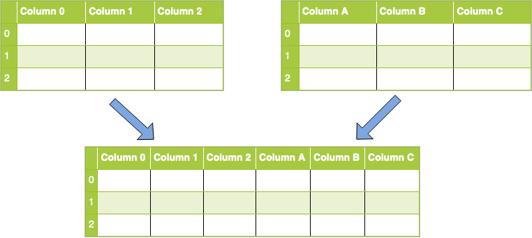
Column Concat

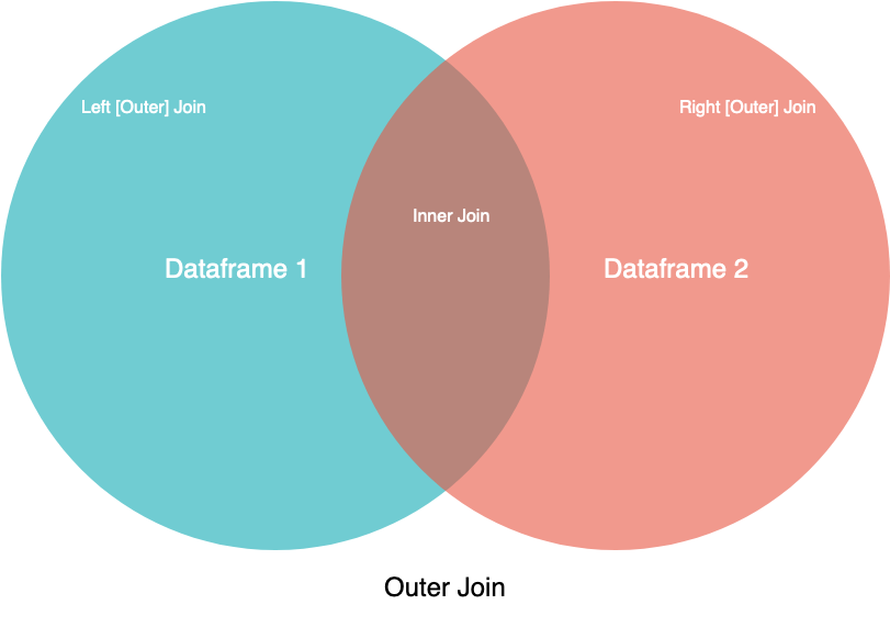
Merge [Inner, Outter (Left, Right)]

concat() for combining DataFrames across rows or columns
- axis represents the axis that you’ll concatenate along.
  - The default value is 0, which concatenates along the index, or row axis.
  - Alternatively, a value of 1 will concatenate vertically, along columns. You can also use the string values "index" or "columns".
- ignore_index defaults to False.
  - If True, then the new combined dataset won’t preserve the original index values in the axis specified in the axis parameter. This lets you have entirely new index values.
merge() for combining data on common columns or indices
- how defaults to inner, but other possible options include outer, left, and right
- on; left_on and right_on specify a column or index that’s present only in the left or right object that you’re merging

# ------------ pd.concat() examples ------------
reindexed = pd.concat(
     [df1, df2], ignore_index=True, axis=1
)
# ------------ pd.merge() examples -------------
pd.merge(
     df1, df2, how="left", on=["col_A", "col_B"]
)
# if left & right DF has diff joining col names
pd.merge(
     df1, df2, how="left", left_on=["col_A1"], right_on=["col_A2"]
)

Numpy

Dense & Sparse Matrix Conversion:
- Sparse → Dense: A.toarray()
Numpy vs Tensor:
- TensorFlow seems to look a lot like NumPy. But here’s something NumPy can’t do: retrieve the gradient of any differentiable expression with respect to any of its inputs.
  - Open a GradientTape scope, apply some computation to one or several input tensors, and retrieve the gradient of the result with respect to the inputs.
- A significant difference between NumPy arrays and TensorFlow tensors is that TensorFlow tensors aren’t assignable: they’re constant

import numpy as np
x = np.ones(shape=(2, 2))
x[0, 0] = 0.

x = tf.ones(shape=(2, 2))
x[0, 0] = 0. # ERROR: fail, as a tensor isn’t assignable.

`sys.path`

sys.path is a built-in variable within the sys module. It contains a list of directories that the interpreter will search in for the required module. When a module(a module is a python file) is imported within a Python file, the interpreter first searches for the specified module among its built-in modules. If not found it looks through the list of directories(a directory is a folder that contains related modules) defined by sys.path.
To locate the installation path of the module: print(module_name.__file__)
Python will locate the module based on the path appears first in sys.path, so in order to change prioritise the installation packages, we can do as follow:

import sys
sys.path.insert(0, '/path/to/site-packages') # location of src

Matplotlib

Set params: plt.rcParams.update({'font.size': 14})
Set the style of the plot plt.style.use('fivethirtyeight') # set at the front of the notebook
- Other styles: seaborn-v0_8-darkgrid

Ax

Set vertical axis range: ax.set_ylim([0,1]) or plt.gca().set_ylim(0,1) #set vertical range to [0-1]
Set horizontal axis range:

Subplots

Enable subplots share the same axis with sharex or sharey: plt.subplots(nrows=3, sharey=True)
fig.tight_layout(pad=2) function of matplotlib allows to adhust the gap between subplots
- pad parameter to specify gap size

Python

assert: to check if the data is expected (assert len(x.shape) == 2) and will raise Exception if not matching.
iter(): return an iterator for the given a list, set, tuple or object with __next__() method.

phones = ['apple', 'samsung', 'oneplus']
phones_iter = iter(phones)
print(next(phones_iter))

os.environ[variable]=value a mapping object that represents the user’s environmental variables.
sys.path is a built-in variable within the sys module. It contains a list of directories that the interpreter will search in for the required module. When a module(a module is a python file) is imported within a Python file, the interpreter first searches for the specified module among its built-in modules. If not found it looks through the list of directories(a directory is a folder that contains related modules) defined by sys.path.
random module
- Randomly select an item in a list: random.randint(0, len_x)
- Randomly select subset of items in a list:
```
# Method 1
indices_permutation = random.permutation(len(x))
dataset[indices_permutation][:10]
# Method 2: select 10 out of the dataset
indices_permutation = random.sample(range(len(trainset)), 10)
dataset[indices_permutation]
```
- Normal distribution with mean 0 and standard deviation 1: np.random.normal(size=(3,1), loc=0., scale=1.)
- Uniform distribution between 0 and 1: np.random.uniform(size=(3, 1), low=0., high=1.)

Day 1

VS Code

VS Code Shortcuts

CMD + Shift + P Command Palette
CMD + P Quickly open files

Auto Venv Activation

# in .vscode settings.json
"python.terminal.activateEnvironment": true

Code Formatter & Linting

The main coding standard for Python is PEP8 (Python Enhancement Proposal 8)
- Linters such as flake8 and pylint highlight places where your code doesn’t conform with PEP8.
- Automatic formatters such as black that will update your code automatically to conform with coding standards.
- Type Checker mypy is a static type checker for Python. Type checkers help ensure that you're using variables and functions in your code correctly. With mypy, add type hints (PEP 484) to your Python programs, and mypy will warn you when you use those types incorrectly.

Setup inside VS Code

How to install flack8:
- Step 1: Install black in virtual environment: pip install flake8
- Step 2: Open the Command Palette (CMD + Shift + P) → Search the “Python: Select Linter” and press enter. Select the “flake8”
How to install black:
- Step 1: Install black in virtual environment: pip install black
- Step 2: Open the Command Palette (CMD + Shift + P) → “Preferences → Settings”
  - Search “format on save” and check the checkbox
  - Search “python formatting provider” and select the black.
- NOTE: can run black seperately black -l 80 --preview src/youtube_statistics.py
How to install isort:
- Open the Command Palette (CMD + Shift + P). Search the “Preferences: Open User Settings (JSON)” and press enter. It will open the “settings.json” and add the follow code into that:
```
"editor.codeActionsOnSave": {
  "source.organizeImports": true
}
```

Setup pre-commit using `git hooks`

This is to ensure the code formatter, linting is running before the commit

install requirements-dev dependencies

# requirements-dev.txt
flake8
black
mypy
coverage

add hooksPath into git config core: git config --local core.hooksPath .git/hooks/

pre-commit file inside .git/hooks/

# content inside pre-commit file
echo "Running lint.sh before commit"
bash lint.sh
echo "Linting completed"

make pre-commit file executable via chmod +x .git/hooks//pre-commit

Define the content in lint.sh

# content inside lint.sh
  linting_path="."
  echo "-------------Formatter with black-----------------"
  black $linting_path --line-length=88

  echo "-------------Linting with flake8-----------------"
  flake8 $linting_path --max-line-length=88 --ignore=E203,W503,E231,E266,E722

  echo "-------------Type checking with mypy-----------------"
  mypy $linting_path  --ignore-missing-imports

Setup pre-commit using `pre-commit` package

Reading

FilesExpand file tree

daily_knowledge.md

Latest commit

History

daily_knowledge.md

File metadata and controls

2024

Day 2

Day 1

Matplotlib

Pandas

.loc vs .iloc

2023

Day 11

Python

Pandas

pd.melt vs contingency table (pd.crosstab)

Matplotlib

Conda vs Pip: Package Availability

Day 10

Pandas

pd.cut vs pd.qcut

.read_csv() by chunk

Python

lru_cache from functools

typing Annotated

Float to Decimal conversion

Day 9

subprocess module

subprocess vs os.system

sys module

Day 8

Matplotlib

Relative import

subprocess.Popen to send Linux command

os.path

List

Day 7

Conda

Conda env creation:

conda create --file requirements.txt vs conda env create --file environment.yml

Other common conda commands

Day 6

Matplotlib

Numpy

Holidays package

Code Refactor

Day 5

Seaborn

Histogram (Displot)

Pairplot

Python

Pandas

Select columns based on Dtype

Time-series

df.query

Check & Remove Duplicates

Matplotlib

Day 4

Numpy

Pandas

groupby

Python

.env

Day 3

Notebook

VScode

Matplotlib

Figure

Python

Day 2

Pandas

Joining Pandas DataFrame with Numpy array

Joining Pandas DataFrame with Pandas Series

Joining Pandas DataFrames

Numpy

sys.path

Matplotlib

Ax

Subplots

`.loc` vs `.iloc`

`pd.melt` vs contingency table (`pd.crosstab`)

`pd.cut` vs `pd.qcut`

`.read_csv()` by chunk

`lru_cache` from `functools`

typing `Annotated`

`subprocess` module

`subprocess` vs `os.system`

`sys` module

`subprocess.Popen` to send Linux command

`os.path`

`conda create --file requirements.txt` vs `conda env create --file environment.yml`

`df.query`

`groupby`

`.env`

`sys.path`

Setup pre-commit using `git hooks`

Setup pre-commit using `pre-commit` package