In the two baseline models, they produce two independent alpha estimates as currently coded while in theory these should be a single shared parameter for the two different likelihoods. While the carbon alpha is informed by the data, the nitrogen alpha posterior produced is purely draws from the supplied beta prior (see reprex below). I do not think it is currently possible to incorporate shared parameters in brms as it stands, but is something the writers are planning to introduce in version 3. The shared alpha parameter model could be coded directly into STAN but I appreciate this will be much more complicated to implement for a package. It is possible that the alpha value could be treated as a missing parameter in d15N that needs to be imputed on the fly in brms, using the mi() functionality (see https://paulbuerkner.com/brms/articles/brms_missings.html)? Something like:
d15n ~ dn * tp - l1 + n1 * mi(ar) + n2 * (1 - mi(ar))
ar | mi() ~ (alpha - min_alpha) / (max_alpha - min_alpha)
Reprex:
library(bayesplot)
library(brms)
library(dplyr)
library(ggdist)
library(grid)
library(tidybayes)
library(tidyr)
library(trps)

### Load in data as per vignette (https://benjaminhlina.github.io/trps/articles/estimate_trophic_position_two_source_model_ar.html#posterior-draws)
con_tsar <- consumer_iso %>%
  arrange(ecoregion, common_name) %>%
  group_by(ecoregion, common_name) %>%
  mutate(
    id = row_number()
  ) %>%
  ungroup() %>%
  dplyr::select(id, common_name:d15n)

b1_tsar <- baseline_1_iso %>%
  arrange(ecoregion, common_name) %>%
  group_by(ecoregion, common_name) %>%
  mutate(
    id = row_number()
  ) %>%
  ungroup() %>%
  dplyr::select(id, ecoregion:d15n_b1)

b2_tsar <- baseline_2_iso %>%
  arrange(ecoregion, common_name) %>%
  group_by(ecoregion, common_name) %>%
  mutate(
    id = row_number()
  ) %>%
  ungroup() %>%
  dplyr::select(id, ecoregion:d15n_b2)

combined_iso_tsar <- con_tsar %>%
  left_join(b1_tsar, by = c("id", "ecoregion")) %>%
  left_join(b2_tsar, by = c("id", "ecoregion"))

combined_iso_tsar_1 <- combined_iso_tsar %>%
  group_by(ecoregion, common_name) %>%
  mutate(
    c1 = mean(d13c_b1, na.rm = TRUE),
    n1 = mean(d15n_b1, na.rm = TRUE),
    c2 = mean(d13c_b2, na.rm = TRUE),
    n2 = mean(d15n_b2, na.rm = TRUE),
    l1 = 2
  ) %>%
  ungroup() %>%
  add_alpha()

# Run model with default priors (a = 1 and b = 1)
model_output_tsar_a1b1 <- brm(
  formula = two_source_model_ar(),
  prior = two_source_priors_ar(),
  stanvars = two_source_priors_params_ar(),
  data = combined_iso_tsar_1,
  family = gaussian(),
  chains = 2,
  iter = 2000,
  warmup = 1000,
  cores = 4,
  seed = 4,
  control = list(adapt_delta = 0.95)
)
#> Compiling Stan program...
#> Start sampling

# Run model with alternative priors (a = 3, b = 2)
model_output_tsar_a3b2 <- brm(
  formula = two_source_model_ar(),
  prior = two_source_priors_ar(),
  stanvars = two_source_priors_params_ar(a = 3, b = 2, bp = TRUE),
  data = combined_iso_tsar_1,
  family = gaussian(),
  chains = 2,
  iter = 2000,
  warmup = 1000,
  cores = 4,
  seed = 4,
  control = list(adapt_delta = 0.95)
)
#> Compiling Stan program...
#> Start sampling

# Extract draws for plotting
post_draws_a1b1 <- model_output_tsar_a1b1 %>%
  gather_draws(b_alpha_ar_Intercept, b_d15n_ar_Intercept) %>% data.frame()

post_draws_a3b2 <- model_output_tsar_a3b2 %>%
  gather_draws(b_alpha_ar_Intercept, b_d15n_ar_Intercept) %>% data.frame()

# Plot histogram of draws plus prior beta distribution
ggplot() +
  geom_histogram(aes(x = post_draws_a1b1[post_draws_a1b1$.variable == "b_alpha_ar_Intercept", ".value"], y = after_stat(density)),
                 col = "#EFA355", fill = "#EFA355", alpha = 0.3) +
  geom_histogram(aes(x = post_draws_a1b1[post_draws_a1b1$.variable == "b_d15n_ar_Intercept", ".value"], y = after_stat(density)),
                 col = "#421E22", fill = "#421E22", alpha = 0.3) +
  geom_line(aes(x = seq(0,1,0.01), y = dbeta(seq(0,1,0.01), 1,1)),
            linewidth = 2, col = "black") +
  labs(x = NULL, y = NULL, subtitle = "Orange = alpha_ar; Brown = d15n_ar, prior = beta(1,1)") +
  theme_bw()
#> `stat_bin()` using `bins = 30`. Pick better value `binwidth`.
#> `stat_bin()` using `bins = 30`. Pick better value `binwidth`.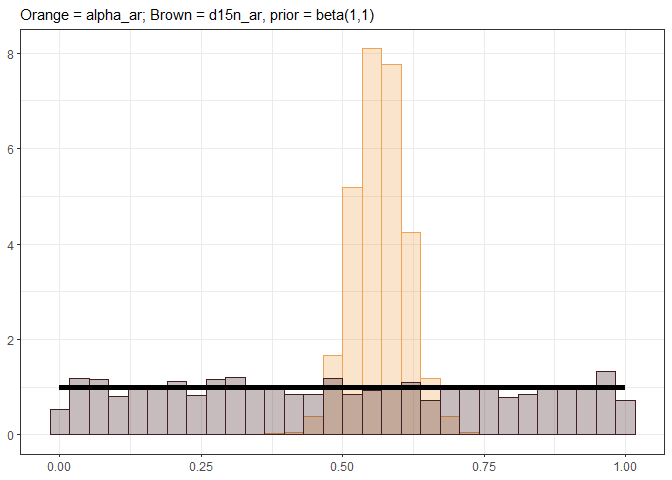
ggplot() +
  geom_histogram(aes(x = post_draws_a3b2[post_draws_a3b2$.variable == "b_alpha_ar_Intercept", ".value"], y = after_stat(density)),
                 col = "#EFA355", fill = "#EFA355", alpha = 0.3) +
  geom_histogram(aes(x = post_draws_a3b2[post_draws_a3b2$.variable == "b_d15n_ar_Intercept", ".value"], y = after_stat(density)),
                 col = "#421E22", fill = "#421E22", alpha = 0.3) +
  geom_line(aes(x = seq(0,1,0.01), y = dbeta(seq(0,1,0.01), 3,2)),
            linewidth = 2, col = "black") +
  labs(x = NULL, y = NULL, subtitle = "Orange = alpha_ar; Brown = d15n_ar, prior = beta(3,2)") +
  theme_bw()
#> `stat_bin()` using `bins = 30`. Pick better value `binwidth`.
#> `stat_bin()` using `bins = 30`. Pick better value `binwidth`.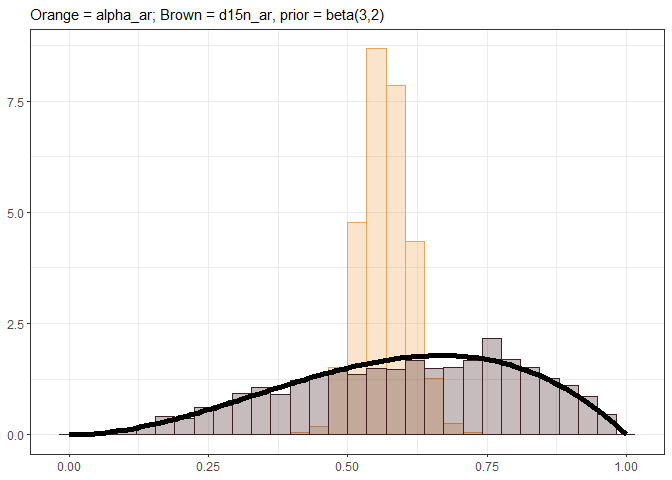
Created on 2025-12-08 with reprex v2.1.1
In the two baseline models, they produce two independent alpha estimates as currently coded while in theory these should be a single shared parameter for the two different likelihoods. While the carbon alpha is informed by the data, the nitrogen alpha posterior produced is purely draws from the supplied beta prior (see reprex below). I do not think it is currently possible to incorporate shared parameters in brms as it stands, but is something the writers are planning to introduce in version 3. The shared alpha parameter model could be coded directly into STAN but I appreciate this will be much more complicated to implement for a package. It is possible that the alpha value could be treated as a missing parameter in d15N that needs to be imputed on the fly in brms, using the mi() functionality (see https://paulbuerkner.com/brms/articles/brms_missings.html)? Something like:
d15n ~ dn * tp - l1 + n1 * mi(ar) + n2 * (1 - mi(ar))
ar | mi() ~ (alpha - min_alpha) / (max_alpha - min_alpha)
Reprex:
Created on 2025-12-08 with reprex v2.1.1