When migration matrix isn't symmetrical (i.e. more migration in one direction than the other), the estimated prevalence and incidence are very different between the two demes, despite the same starting conditions. This pattern is consistent across multiple seeds and repeated runs of the model.
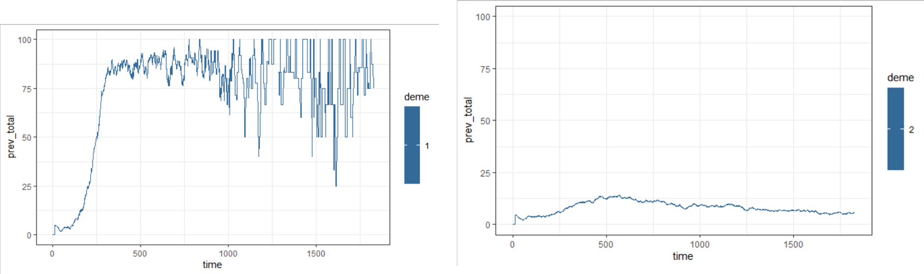
In addition when using the sim_haplotype_tree() function, an error is returned :
Error in sim_haplotype_tree_cpp(args) :
human host receives infectious bite from mosquito that has not yet been infected
This error is generated on line 248 of main.cpp, occurs when mosquito_pop.count(mosquito_ID[i]) == 0
This may be simply due to the population declining in one deme and growing in the other and may want to think about writing something into the code to replenish populations, or could also be an additional bug to investigate.
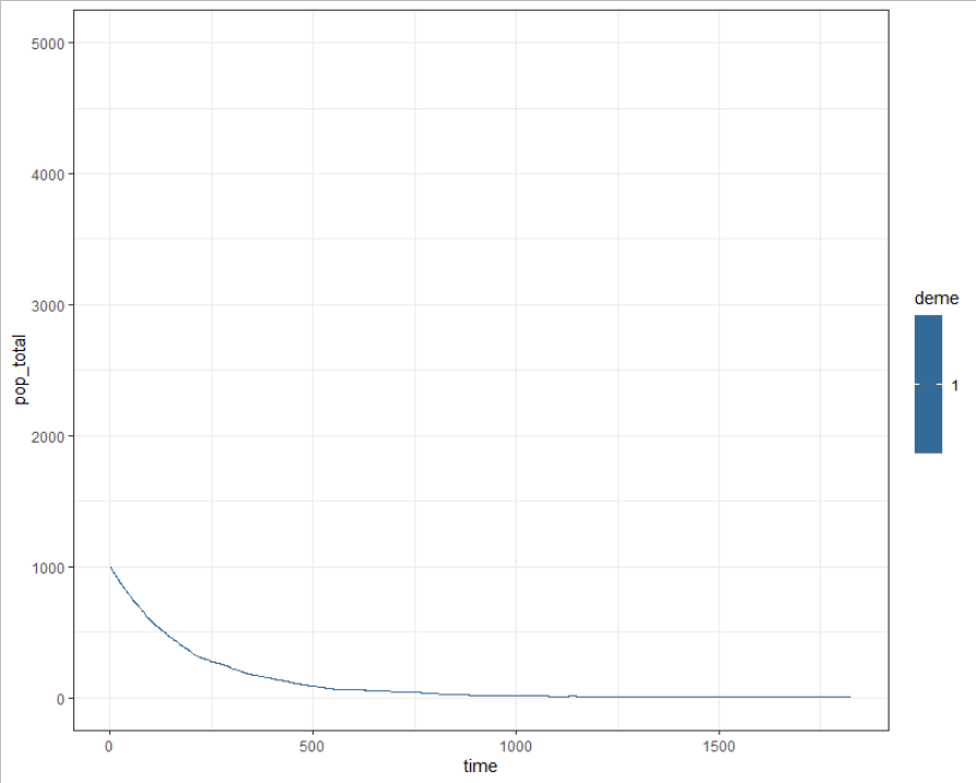
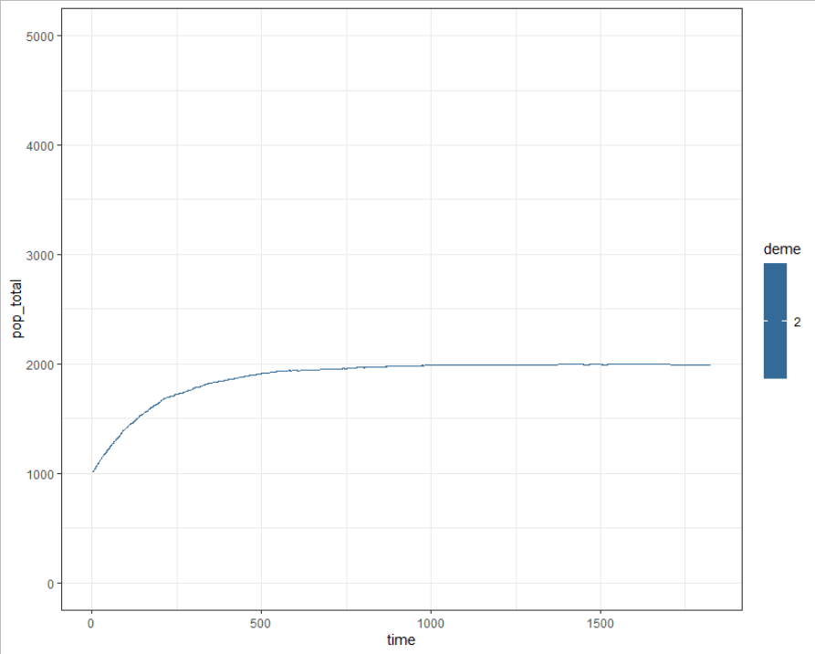
Code to generate error
`
library(devtools)
devtools::install_github("mrc-ide/SIMPLEGEN", ref= "develop")
library(SIMPLEGEN)
library(ggplot2)
library(dplyr)
library(tidyverse)
Changing migration between two demes
define a migration matrix as done in vignette
m <- 0.005
mig_mat <- rbind(c(1 - m, m),
c(0.0, 1.0))
create project and define model parameters
s <- simplegen_project() %>%
define_epi_model_parameters(H = c(1e3,1e3),
M = c(1e4,1e4),
seed_infections = c(50,50),
prob_acute = 0.5,
mig_mat = mig_mat,
detectability_microscopy_acute = 1,
detectability_microscopy_chronic = 1,
detectability_PCR_acute = 1,
detectability_PCR_chronic = 1,
treatment_seeking_mean = 0.2)
define daily sampling
daily_df <- rbind(data.frame(name = "prev_acute", deme = c(1,2), state = "A", measure = "prevalence", diagnostic = "true", age_min = 0, age_max = 100),
data.frame(name = "prev_chronic", deme = c(1,2), state = "C", measure = "prevalence", diagnostic = "true", age_min = 0, age_max = 100),
data.frame(name = "inc_acute", deme = c(1,2), state = "A", measure = "incidence", diagnostic = "true", age_min = 0, age_max = 100),
data.frame(name = "inc_chronic", deme = c(1,2), state = "C", measure = "incidence", diagnostic = "true", age_min = 0, age_max = 100),
data.frame(name = "count_acute", deme =c(1,2), state = "A", measure = "count", diagnostic = "true", age_min = 0, age_max = 5),
data.frame(name = "count_H", deme =c(1,2), state = "H", measure = "count", diagnostic = NA, age_min = 0, age_max = 100))
define sweeps
max_time <- 365 * 5
sweep_df <- rbind(data.frame(name = "prev_acute", time = max_time, deme = c(1,2), measure = "prevalence", state = "A", diagnostic = "true", age_min = seq(0, 100, 1), age_max = seq(0, 100, 1) + 1),
data.frame(name = "prev_chronic", time = max_time, deme = c(1,2), measure = "prevalence", state = "C", diagnostic = "true", age_min = seq(0, 100, 1), age_max = seq(0, 100, 1) + 1),
data.frame(name = "inc_acute", time = max_time, deme = c(1,2), measure = "incidence", state = "A", diagnostic = "true", age_min = seq(0, 100, 1), age_max = seq(0, 100, 1) + 1),
data.frame(name = "inc_chronic", time = max_time, deme = c(1,2), measure = "incidence", state = "C", diagnostic = "true", age_min = seq(0, 100, 1), age_max = seq(0, 100, 1) + 1))
define surveys
survey_df <- data.frame(t_start = 600, t_end = 650, reporting_interval = 7, deme = c(1,2), measure = "prevalence", sampling = NA, diagnostic = "true", age_min = 0, age_max = 100, sample_size = 100)
load sampling parameters into project
s <- define_epi_sampling_parameters(project = s,
daily = daily_df,
# sweeps = sweep_df,
surveys = survey_df)
simulate from transmission model
set.seed(12)
s <- s %>%
sim_epi(max_time = max_time,
save_transmission_record = TRUE,
transmission_record_location = "ignore/trans_record.csv",
overwrite_transmission_record = TRUE,
silent = FALSE)
plots for each deme
s$epi_output$daily %>%
dplyr::filter(name %in% c("count_H")) %>%
dplyr::group_by(time,deme) %>%
dplyr::filter(deme == 1) %>%
dplyr::summarise(pop_total = sum(value)) %>%
ggplot() + theme_bw() +
geom_line(aes(x = time, y = pop_total, col = deme)) +
ylim(c(0,5000))
s$epi_output$daily %>%
dplyr::filter(name %in% c("count_H")) %>%
dplyr::group_by(time,deme) %>%
dplyr::filter(deme == 2) %>%
dplyr::summarise(pop_total = sum(value)) %>%
ggplot() + theme_bw() +
geom_line(aes(x = time, y = pop_total, col = deme)) +
ylim(c(0,5000))
s$epi_output$daily %>%
dplyr::filter(name %in% c("prev_acute", "prev_chronic")) %>%
dplyr::group_by(time,deme) %>%
dplyr::filter(deme == 1) %>%
dplyr::summarise(prev_total = sum(value)) %>%
ggplot() + theme_bw() +
geom_line(aes(x = time, y = prev_total, col = deme)) +
ylim(c(0,100))
s$epi_output$daily %>%
dplyr::filter(name %in% c("prev_acute", "prev_chronic")) %>%
dplyr::group_by(time,deme) %>%
dplyr::filter(deme == 2) %>%
dplyr::summarise(prev_total = sum(value)) %>%
ggplot() + theme_bw() +
geom_line(aes(x = time, y = prev_total, col = deme)) +
ylim(c(0,100))
prune transmission record
s <- prune_transmission_record(project = s,
transmission_record_location = "ignore/trans_record.csv")
define genetic parameters
s <- define_genetic_params(s)
simulate relatedness
set.seed(1)
s <- sim_haplotype_tree(project = s,
silent = FALSE)
`
When migration matrix isn't symmetrical (i.e. more migration in one direction than the other), the estimated prevalence and incidence are very different between the two demes, despite the same starting conditions. This pattern is consistent across multiple seeds and repeated runs of the model.

In addition when using the sim_haplotype_tree() function, an error is returned :
Error in sim_haplotype_tree_cpp(args) :
human host receives infectious bite from mosquito that has not yet been infected
This error is generated on line 248 of main.cpp, occurs when mosquito_pop.count(mosquito_ID[i]) == 0
This may be simply due to the population declining in one deme and growing in the other and may want to think about writing something into the code to replenish populations, or could also be an additional bug to investigate.
Code to generate error
`
library(devtools)
devtools::install_github("mrc-ide/SIMPLEGEN", ref= "develop")
library(SIMPLEGEN)
library(ggplot2)
library(dplyr)
library(tidyverse)
Changing migration between two demes
define a migration matrix as done in vignette
m <- 0.005
mig_mat <- rbind(c(1 - m, m),
c(0.0, 1.0))
create project and define model parameters
s <- simplegen_project() %>%
define_epi_model_parameters(H = c(1e3,1e3),
M = c(1e4,1e4),
seed_infections = c(50,50),
prob_acute = 0.5,
mig_mat = mig_mat,
detectability_microscopy_acute = 1,
detectability_microscopy_chronic = 1,
detectability_PCR_acute = 1,
detectability_PCR_chronic = 1,
treatment_seeking_mean = 0.2)
define daily sampling
daily_df <- rbind(data.frame(name = "prev_acute", deme = c(1,2), state = "A", measure = "prevalence", diagnostic = "true", age_min = 0, age_max = 100),
data.frame(name = "prev_chronic", deme = c(1,2), state = "C", measure = "prevalence", diagnostic = "true", age_min = 0, age_max = 100),
data.frame(name = "inc_acute", deme = c(1,2), state = "A", measure = "incidence", diagnostic = "true", age_min = 0, age_max = 100),
data.frame(name = "inc_chronic", deme = c(1,2), state = "C", measure = "incidence", diagnostic = "true", age_min = 0, age_max = 100),
data.frame(name = "count_acute", deme =c(1,2), state = "A", measure = "count", diagnostic = "true", age_min = 0, age_max = 5),
data.frame(name = "count_H", deme =c(1,2), state = "H", measure = "count", diagnostic = NA, age_min = 0, age_max = 100))
define sweeps
max_time <- 365 * 5
sweep_df <- rbind(data.frame(name = "prev_acute", time = max_time, deme = c(1,2), measure = "prevalence", state = "A", diagnostic = "true", age_min = seq(0, 100, 1), age_max = seq(0, 100, 1) + 1),
data.frame(name = "prev_chronic", time = max_time, deme = c(1,2), measure = "prevalence", state = "C", diagnostic = "true", age_min = seq(0, 100, 1), age_max = seq(0, 100, 1) + 1),
data.frame(name = "inc_acute", time = max_time, deme = c(1,2), measure = "incidence", state = "A", diagnostic = "true", age_min = seq(0, 100, 1), age_max = seq(0, 100, 1) + 1),
data.frame(name = "inc_chronic", time = max_time, deme = c(1,2), measure = "incidence", state = "C", diagnostic = "true", age_min = seq(0, 100, 1), age_max = seq(0, 100, 1) + 1))
define surveys
survey_df <- data.frame(t_start = 600, t_end = 650, reporting_interval = 7, deme = c(1,2), measure = "prevalence", sampling = NA, diagnostic = "true", age_min = 0, age_max = 100, sample_size = 100)
load sampling parameters into project
s <- define_epi_sampling_parameters(project = s,
daily = daily_df,
# sweeps = sweep_df,
surveys = survey_df)
simulate from transmission model
set.seed(12)
s <- s %>%
sim_epi(max_time = max_time,
save_transmission_record = TRUE,
transmission_record_location = "ignore/trans_record.csv",
overwrite_transmission_record = TRUE,
silent = FALSE)
plots for each deme
s$epi_output$daily %>%
dplyr::filter(name %in% c("count_H")) %>%
dplyr::group_by(time,deme) %>%
dplyr::filter(deme == 1) %>%
dplyr::summarise(pop_total = sum(value)) %>%
ggplot() + theme_bw() +
geom_line(aes(x = time, y = pop_total, col = deme)) +
ylim(c(0,5000))
s$epi_output$daily %>%
dplyr::filter(name %in% c("count_H")) %>%
dplyr::group_by(time,deme) %>%
dplyr::filter(deme == 2) %>%
dplyr::summarise(pop_total = sum(value)) %>%
ggplot() + theme_bw() +
geom_line(aes(x = time, y = pop_total, col = deme)) +
ylim(c(0,5000))
s$epi_output$daily %>%
dplyr::filter(name %in% c("prev_acute", "prev_chronic")) %>%
dplyr::group_by(time,deme) %>%
dplyr::filter(deme == 1) %>%
dplyr::summarise(prev_total = sum(value)) %>%
ggplot() + theme_bw() +
geom_line(aes(x = time, y = prev_total, col = deme)) +
ylim(c(0,100))
s$epi_output$daily %>%
dplyr::filter(name %in% c("prev_acute", "prev_chronic")) %>%
dplyr::group_by(time,deme) %>%
dplyr::filter(deme == 2) %>%
dplyr::summarise(prev_total = sum(value)) %>%
ggplot() + theme_bw() +
geom_line(aes(x = time, y = prev_total, col = deme)) +
ylim(c(0,100))
prune transmission record
s <- prune_transmission_record(project = s,
transmission_record_location = "ignore/trans_record.csv")
define genetic parameters
s <- define_genetic_params(s)
simulate relatedness
set.seed(1)
s <- sim_haplotype_tree(project = s,
silent = FALSE)
`