The overall process in this session is mainly based on the TwoSampleMR in R vignette.
The following contents were tested on GSDS Cluster.
To avoid conflicts in dependecies, we will create new environment for two sample MR (twoMR) in this session. First, lets install R and devtools in new conda environment (Already installed in gsds cluster under leelabguest)
conda create -n twoMR r-base r-essentials r-devtools r-remotes r-gmp -c conda-forge -c R
conda activate twoMR ; R --no-save
TwoSampleMR pacakge is installed from github
remotes::install_github("MRCIEU/TwoSampleMR")
The workflow for performing MR is as follows:
c. Harmonise the effect sizes for the instruments on the exposures and the outcomes to be each for the same reference allele
The IEU GWAS database (IGD) contains complete GWAS summary statistics from a large number of studies. You can browse them through the website.
From the package, available_outcomes() will list up outcomes obtainable from IEU.
ao <- available_outcomes()
head(ao)
In this part of session, we will follow the example from the package using formatted summary statistics.
We want to discover causal relationship between BMI and CHD. \
BMI comes from GIANT Consortium
CHD is from CARDIoGRAMplusC4D.
bmi_exp_dat <- extract_instruments(outcomes = 'ieu-a-2')
head(bmi_exp_dat)
The output from this function is a new data frame with standardised column names: \
- SNP
- exposure
- beta.exposure
- se.exposure
- effect_allele.exposure
- other_allele.exposure
- eaf.exposure
- mr_keep.exposure
- pval.exposure
- pval_origin.exposure
- id.exposure
- data_source.exposure
- units.exposure
- gene.exposure
- samplesize.exposure
Following similar procedure as Exposure data acquirment, let's bring CHD summary statistics. By taking snps argument, we can scope the common variant list with BMI
chd_out_dat <- extract_outcome_data(
    snps = bmi_exp_dat$SNP,
    outcomes = 'ieu-a-7'
)
head(chd_out_dat)
Harmonizing data step is required because there are mismatches between alleles in exposure and outcome. Recent GWASs typically present the effects of a SNP in reference to the allele on the forward strand but not necessarily.
dat <- harmonise_data(
    exposure_dat = bmi_exp_dat,
    outcome_dat = chd_out_dat
)
There are three options to harmonising the data.
- Assume all alleles are presented on the forward strand
- Try to infer the forward strand alleles using allele frequency information
- Correct the strand for non-palindromic SNPs, but drop all palindromic SNPs
By default, the harmonise_data function uses option 2, but this can be modified using the action argument, e.g. harmonise_data(exposure_dat, outcome_dat, action = 3).
Before we perform MR, lets find out which method is available in the package
mr_method_list()
Let's try MR with Egger, two sample maximum likelihood,simple median, and IVW. You can add list of methods or methods set by default.
res <- mr(dat, method_list = c("mr_egger_regression", "mr_two_sample_ml","mr_simple_median","mr_ivw"))
res
Some Methods can perform sensitivity test which are implemented in mr_heterogeneity()
mr_heterogeneity(dat)
Intercept tern in MR egger regression indicate the presence of Horizontal Pleiotropy.
mr_pleiotropy_test(dat)
Single SNP MR can be also performed by following.
res_single <- mr_singlesnp(dat)
head(res_single)
To see if a single snp is driving the association, we can perform leave-one-out MR. In this case, we can see that there is no single variant that driving the association between exposure and outcome.
res_loo <- mr_leaveoneout(dat)
head(res_loo)
Visualizing MR analysis with plot can be performed as below: Let's save to pdf using ggsave() from ggplot2
res <- mr(dat)
p1 <- mr_scatter_plot(res, dat)
print(length(p1))
ggplot2::ggsave(p1[[1]], file = "/home/n1/leelabguest/GCDA/4_MR/results/example_Scatter.png", width = 7, height = 7)
Download the plot to local computer.
scp leelabguest@147.47.200.192:/home/n1/leelabguest/GCDA/4_MR/results/example_Scatter.png ./
Let's try two-sample MR between HDL exposure and Diabetes outcome
HDL Exposure data from IEU GWAS
HDL_exp_dat <- extract_instruments(outcomes = 'ieu-a-299')
head(HDL_exp_dat)
Diabetes outcome data downloaded from Pheweb
The downloaded summary statistics on Diabetes Malitious from KoGES pheweb is located in ~/GCDA/4_MR/data
It is saved as tab-delimited format(.tsv), we can take a look.
manual outcome data frame should include snps, beta, effect, se, alleles, eaf column.
Since we have case af and control af, we can generate eaf.
library(data.table)
library(dplyr)
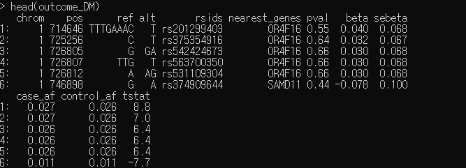
outcome_DM = fread('/home/n1/leelabguest/GCDA/4_MR/data/phenocode-KoGES_DM.tsv')
head(outcome_DM)
outcome_DM = outcome_DM %>% mutate(eaf = (case_af*5083+control_af*67127)/72210,n = 72210,pheno = "DM")
SNP columns
outcome_dat <- format_data(
    type="outcome",
    phenotype_col="pheno",
    dat = outcome_DM,
    snps = HDL_exp_dat$SNP,
    snp_col = "rsids",
    beta_col = "beta",
    se_col = "sebeta",
    effect_allele_col = "ref",
    other_allele_col = "alt",
    eaf_col = "eaf",
    samplesize_col = "n"
)
dat <- harmonise_data(
    exposure_dat = HDL_exp_dat,
    outcome_dat = outcome_dat
)
res = mr(dat)
res
p1 <- mr_scatter_plot(res, dat)
ggplot2::ggsave(p1[[1]], file = "/home/n1/leelabguest/GCDA/4_MR/results/HDL_T2D_Scatter.png", width = 7, height = 7)
Heterogeneity test indicates there is a presence of heterogeneity between exposure and outcome,
which is reasonable since the population group is different (Global vs KOR)
mr_heterogeneity(dat)
There is a slight evidence of horizontal pleiotropy
mr_pleiotropy_test(dat)
Single SNP MR can be also performed by following. We can visualize the results via forest and funnel plots
res_single <- mr_singlesnp(dat)
head(res_single)
p2 <- mr_forest_plot(res_single)
ggplot2::ggsave(p2[[1]], file = "/home/n1/leelabguest/GCDA/4_MR/results/HDL_T2D_Forest.png", width = 7, height = 7)
p3 <- mr_funnel_plot(res_single)
ggplot2::ggsave(p3[[1]], file = "/home/n1/leelabguest/GCDA/4_MR/results/HDL_T2D_Funnel.png", width = 7, height = 7)
To see if a single snp is driving the association, we can perform leave-one-out MR. In this case, we can see that there is no single variant that driving the association between exposure and outcome.
res_loo <- mr_leaveoneout(dat)
head(res_loo) ; summary(res_loo$p)
p4 <- mr_leaveoneout_plot(res_loo)
ggplot2::ggsave(p4[[1]], file = "/home/n1/leelabguest/GCDA/4_MR/results/HDL_T2D_LOO.png", width = 7, height = 7)
This Section is based on MVMR package vignette.
