Previous Lesson: FCND - 02 - Planning This Lesson: FCND - 03 - Control Next Lesson: +FCND - 04 - Estimation
Forces and Moments omega (w) is the rotation rate measured in radians per second. 2pi is 1 rotation per second. The thrust and the induced moment are proportional to w^2.


k is the constant of proportionality between the forces and moments. Depends on the size of the blades and the air density.

Causes rotational acceleration. Moment of Inertia can be different for each axis. Moment is Torque. psi is yaw.


4 variables are required for motion in 1 dimension (here it is up and down, z axis translation)

Uncotrolled Drone Exercise If you were to ignore the yaw inducing moments from each motor the state would look like this


Bicopter

Coaxial copter

We use u for control input

Double integrator systems are unstable systems Small mass errors compound quadratically and cause huge errors. Below shows equations to integrate with respect to time. The three types of errors are Model Error, Disturbance & Measurement Noise


Correct Answer:

Simple controller that is proportional to the error. K(sub)p is called P Gain. It is the proportion. We can compute the u_bar (desired acceleration) required easily with the formula from above.

P controllers are already better than the open loop controllers. But
- Oscillations
- Offset

It’s impossible to eliminate the oscillations by just tuning K_p. Also, the higher the oscilation frequency.

This is why we need PD Controllers

We need to look at the rate of change of the error, i.e. the derivative.

The K_p is responsible for matching the target position The K_d is responsible for matching the target velocity

e_dot is the difference between the target speed and the actual speed.
Sometimes PD is enough, but when target changes a lot, we need to tell the desired acceleration, i.e. the derivative of the velocity, z_dot_dot. In an ideal world, z_dot_dot (acceleration) would dictate position exactly and errors would be zero.

This turns out to be the differential equation of a spring whose amplitude is modified by a decaying exponential.

Now using an oscilation and decay function and multiplying them together, we can solve the above differential.

Turns out delta (d) is the damping ration and omega (w) is the natural oscilation frequency and below are the relationships with the proportions.

And this is the result

A big value (close to 1) of damping ratio (delta) yields to a faster decay. A smaller value (close to 0) constitutes, instead, a slower decay. A big value of natural frequency (omega) causes high frequency oscillations. Smaller values of omega, instead, reduce the oscillations' amplitude. The behavior of the PD controller's equation is a sinusoidal oscillation, whose amplitude is modified by a decaying exponential.

Rise time is bound by actuator constraints A system has settled when the oscillations are within +/-2% target value
- To increase the rise time, you have to increase the natural frequency (omega)
- When dampening is 1, there is no overshoot, but rise time is longer
- When dampening is 0.7, rise time is lower but more overshoot
- Larger frequency is small rise and small settle time but ensure control stays within the actuation limits.
- Time constant is T = 1/omega
- Trise = 1.57T

Tuning a system depends on the situation and the characteristics of the system. The video provides you with some guidelines on how to approach the tuning process.
A good practice is to start with the requirements that you need for your system, such as speed, accuracy, stability, etc.
Precisely how you want the system to behave over time (therefore focusing on T-rise and overshoot) and the frequencies (bandwidth and damping ratio).
For example, if you want to reduce T-rise, you can increase the value of the P-gain (Kp). On the other hand, increasing the D-gain (Kd) decreases overshoot and improves the stability.
Here below a reference of how different Kp, Kd values can affect the time domain of the system.

Systematic bias (offset) is introduced when there is a mass error. You can never correct for this with just a PD controller. You need a PID Control.

The integral (area under the curve) accumulates error and counters it.

This is the full PID formula

It is now possible to use just T time constant and d delta damping value.

Saturation limits the ability of the actuator to follow a given command. This limit affects the integral part of the PID controller.

Integral Windup and Clamping When the commanded thrust accumulates due to error accumulated from saturation. The area between the commanded thrust and the engine limitation thrust is called “integral windup”.

We can stop this with “clamping” which turns off the integrator when it is not working.
http://www.20sim.com/webhelp/library_signal_control_pid_control_antiwindup.php
These lessons ignore yaw. yz movement requires vertical thrust (u_1) and torque (u_2) about the x-axis


There are 2 control inputs and they cannot be used to control all three degrees of freedom. This is called an underactuated system. So we sacrifice phi in this lesson and focus on yz control.

In fact a quadrotor system can only control 4 degrees of freedom out of 6 and has to sacrifice some in favor of roll and pitch control.

Linear approximations are used in robotics all the time. We would like to make the non-linear equations into linear differential questions since there are huge advantages to that.

The equation for a linearization of a quadratic function around an operating point is
- f(x_op) → the value of the function at the operating point
- f’(x)|_x=x_op → slope of the tangent line at the operating point
- the deviation from the operating point delta x.
f(x_op) + f’(x)|_x=x_op * (delta)x


At hover, through linearization you can simplify our non-linear set of equations for 2D dynamics as follows:
y_dot_dot sin(phi) = theta

z_dot_dot cos(phi) = 1

simplify y_dot_dot even more: y_dot_dot = g * (delta)phi

This is now fully decoupled from u_1
Vertical acceleration (u_1_bar) affects vertical velocity and position

we can control y through phi. u_2_bar is the 4th derivative of the y position

In case you don't like seeing four dots above your variables, another way of writing the equations you saw in the video is as follows:

Since angular acceleration is the 4th derivative of y position, a small mass error quadruples the position error.


In the 1-dimensional case, measure z position and z velocity and feed into PID to give a vertical thrust command.

u_2 is used to control phi and phi is used to control y Use a cascade when there are multiple loops operating at different timescales. The y controller is a slow controller (10Hz), it commands a phi to the inner controller (100Hz - 1000Hz).

Practical use case of inner + outer loop GPS outdoors or vision indoors is 10Hz so we use an IMU to measure phi at 100Hz - 100 then close the loop every 10Hz.
The outer loop relies on the inner loop being complete at outer loop execution time. This is why the inner loop must be at a faster refresh rate than the outer.
Now we convert the linearized controller to a non-linear controller. We have to recouple the z and y motions by passing the commanded thrust to the y controller also. The z thrust does impact the y position so we need to account for this.


We have to keep track of the vehicle attitude (rotation) and use Euler angles to translate between body and world. Ultimately we want to control the drone in the world frame. Some sensors, e.g. IMU which measures turn rates in the body frame, needs conversion. Some don’t if they are already measured in the world frame.

Orientation = euler angels or quaternions Body rates = rotation rates of each axis, p is z-axis rotation rate.
These "body rate" variables p,q,rp,q,r can be a little confusing. A few things to note about them: 1. The "p" has nothing to do with pitch!
And r has nothing to do with roll!
These three letters were just chosen because they occur sequentially in the alphabet, just like x, y, and z. In fact, p gives the angular rotation rate about the x-axis (in the body frame), q gives the rotation rate about the y-axis (body frame) and r gives the rotation rate about the z-axis (again, in the body frame).
2. They aren't the same as the Euler angle rates of change ϕ˙,θ˙,ψ˙.
While both of these give some sort of angular rate of change, the body rates are calculated in the body frame of the vehicle while the Euler angles are expressed in the world frame.
3. They really are body RATES!
Even though they don't have dots over them. This means that *p*˙,*q*˙,*r*˙ actually express rotational *accelerations*.
p q r are measured in rads per second
In this exercise we see how rotor rotations translate to controls. Controls can be seen as collective force and moments about axes.

and using a rotation matrix we can see rotational acceleration and after two time integrals to advance the translation of the vehicle.

Calculate rotor velocities from controller signals: collective thrust and angular acceleration
https://www.overleaf.com/project/5c582ebf443d3b18312a66e5
Forces come from angular velocities of rotors

Moments around axes come from forces multiplied by shaft length

Set angular velocities based on vertical acceleration, roll, pitch, yaw controls like so


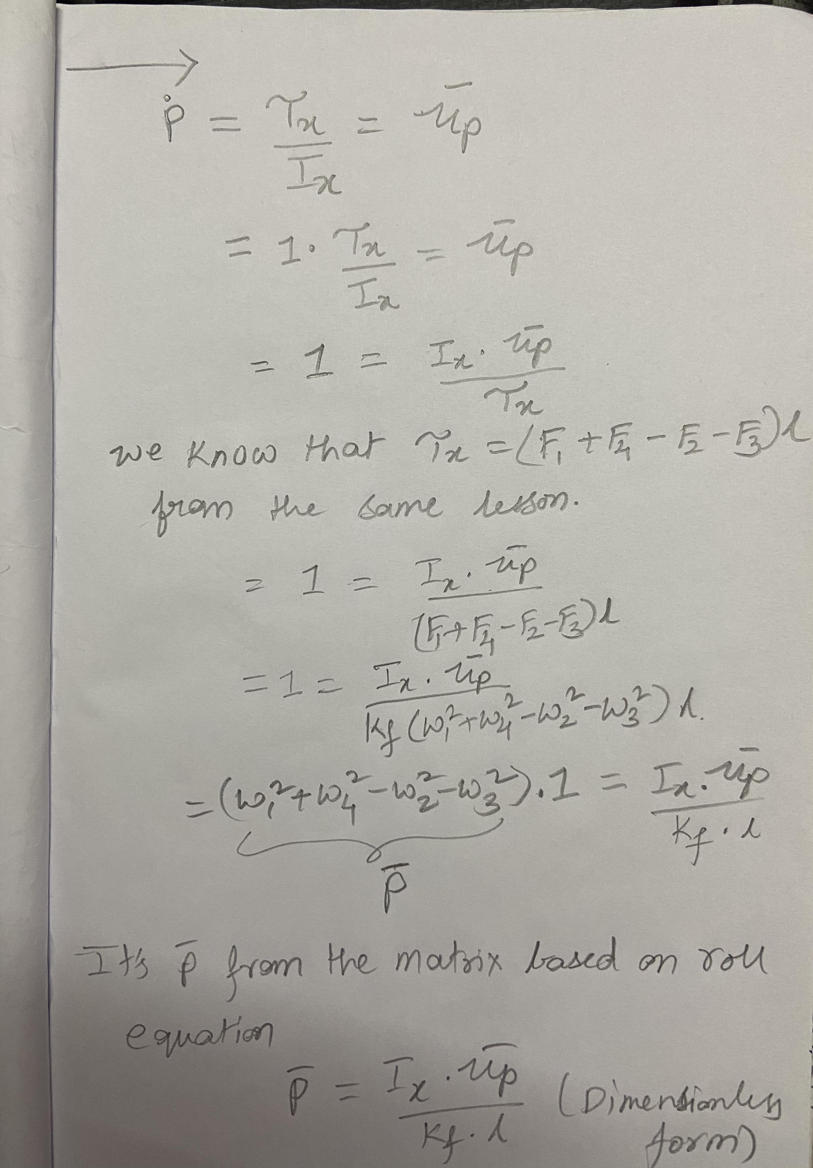
Solving the equations for Dimensionless versions of pqr_bar
Rotation matrix to transform between body-frame accelerations and world-frame accelerations

Linear accelerations

In this lesson we will learn how to use differential thrusts to cause rotational accelerations

- calculate rotational accelerations in the vehicle’s own body frame
- integrate to find the rotational velocities required
- Use math to convert to world-frame phi_dot, theta_dot, psi_dot
- integrate to get the final Euler angles in the world-frame attitude representation
The moments equation below only works in the world frame. We want to calculate accelerations in the body frame because this is where our sensors are.

Need to multiply matricies with the cross product

Euler’s Rotation Equations 𝐌=𝐈𝜔˙+𝜔×(𝐈𝜔)

Cross Product The cross product shows up in Euler's equations. It's a way of multiplying two vectors. If you have two vectors a and b with an angle of θ between them, then the cross product is given by a×b=c, where c is a vector that's perpendicular to both a and b. The direction of this c vector is given by the right hand rule and the magnitude (size) is given by the following equation:
∣**c**∣=∣**a**∣ ∣**b**∣sin(*θ*)
If you want to learn more, you can check out the wikipedia article on the cross product. It's very good!
The angular acceleration in body frame can be calculated using the following equation. The expanded version is provided below as well. Where 𝑝p is a rate of roll in the body frame, 𝑞q is a rate of pitch in body frame and 𝑟r is the rate of yaw. All of these are measured in radians per second

With the last lesson we were able to integrate the rotational rates to get angular velocities. Now we need to update euler angles in the world frame. But they cannot be directly integrated. We need more math.

To go from rotation rates in the body frame to turn rates in the world frame you need this equation. This is for euler representation of attitude, not quaternions.


This link has the equivalent equation for quaternions: https://www.astro.rug.nl/software/kapteyn/_downloads/attitude.pdf
This is done for calculating world-frame attitude.

This lesson is so in-depth and important that its best just to watch the video
https://www.youtube.com/watch?v=CsN5-lHcxyM&
This lesson points to a paper on feed-forward technique for following iterative paths, could be useful for fixed-wing loiter paths:
equations 2,3,4,5,6


This video explains the math from the paper. But in our project, tau_r_p (time constant) is not used, instead we use a p controller and apply a constant kpBank to the b error.
https://www.youtube.com/watch?v=1g_uyhDgoiQ&
Important Equations

Where


Next, we will implement the controller for the drone which will be able to control it in the 3D environment. From lesson, you are already familiar with the architecture of the controller. It consists of altitude controller, position controller, and attitude controller.

The attitude controller breaks down into smaller controllers responsible for roll-pitch, yaw, and body rate.

Parameters which will be required to create the controller are:
- Altitude controller: 𝑘𝑝−𝑧, 𝑘𝑑−𝑧
- Position (lateral) controller: 𝑘𝑝−𝑥, 𝑘𝑑−𝑥, 𝑘𝑝−𝑦, 𝑘𝑑−𝑦
- Roll-Pitch controller: 𝑘𝑝−𝑟𝑜𝑙𝑙, 𝑘𝑝−𝑝𝑖𝑡𝑐ℎ
- Yaw controller: 𝑘𝑝−𝑦𝑎𝑤
- Body rate controller: 𝑘𝑝−𝑝, 𝑘𝑝−𝑞, 𝑘𝑝−𝑟 Based on input parameters we also can calculate 𝛿 and 𝜔𝑛 for altitude 𝑧 and lateral controls 𝑥 and 𝑦.
Note that we are using a slightly different control architecture than what is discussed in the lesson (and what you will implement in the final project).
For now, the job of the lateral controller is to generate commanded values for the rotation matrix elements 𝐑13 (also referred to as 𝑏𝑥) and 𝐑23 (also referred to as 𝑏𝑦).
4.1 Lateral controller The lateral controller will use a PD controller to command target values for elements of the drone's rotation matrix. The drone generates lateral acceleration by changing the body orientation which results in non-zero thrust in the desired direction. This will translate into the commanded rotation matrix elements 𝑏𝑥𝑐 and 𝑏𝑦𝑐. The control equations have the following form:

for the 𝑦 direction the control equations will have the same form as above
The roll-pitch controller is a P controller responsible for commanding the roll and pitch rates (𝑝𝑐 and 𝑞𝑐) in the body frame. First, it sets the desired rate of change of the given matrix elements using a P controller. Note - subscript c means "commanded" and a means "actual”

converted to angular velocities like so:

Body Rate Controller The commanded roll, pitch, and yaw are collected by the body rate controller, and they are translated into the desired rotational accelerations along the axis in the body frame.

notarize.com obefitness.com bloomscape hooked.co boulevard 100thieves airspacelink golinks.io svtrobotics copilot.money density.io - fav founders, highy recommended umba dreamcraft - nocode for gaming bigbrain - fanduel guy welcome - onboarding for employees punchlist.com - employee #7 at square, highly recommended