This work proposes a computer vision model based on the sequential implementation of machine learning models for the detection and reading of U-tube manometers, named VisionGauge. The solution is composed of two stages: a detector and a regressor.

The detector architecture was selected based on an evaluation among YOLOv8s, YOLO11s, and YOLO26s, while the regressor was defined through a comparative study among ResNet-18, EfficientNet-B0, MobileNetV3 Small, and MobileNetV3 Large architectures, all adapted for the regression task.

Custom datasets were created for model training and for the complete evaluation of VisionGauge.

The best configuration was achieved with YOLOv8s + EfficientNet-B0, reaching an F1-Score of 99.94% and an MAE of on the test set, indicating a low regression error.

---

---

Contents

• Read the Paper
• How to Use
  • PyPi Example
  • VisionGauge API
  • Python API Request
• Citation
• References

How to Use

PyPi Example:

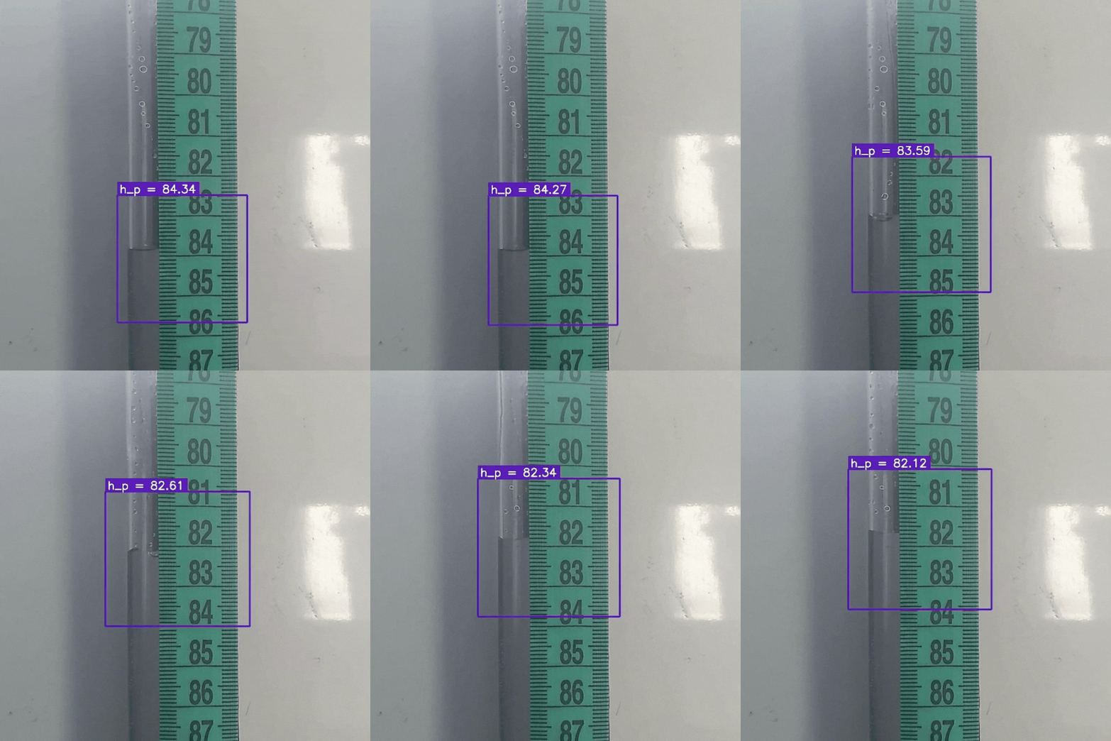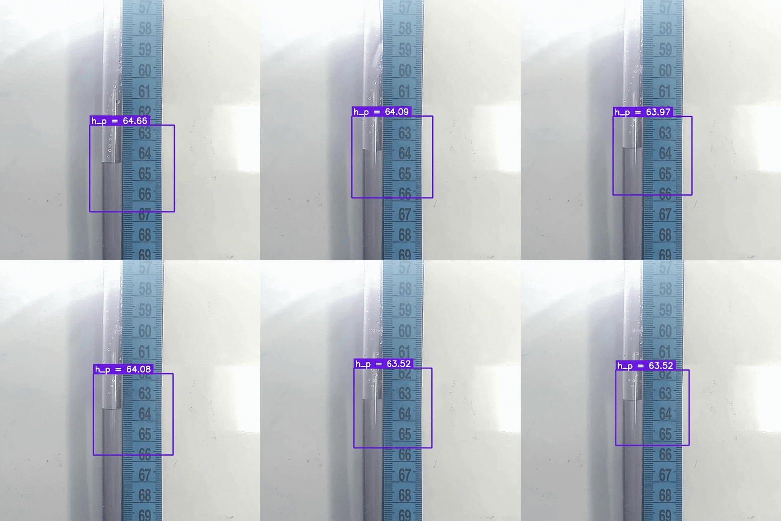The first step you must take for PyPI inference is to install the library as follows:

!pip install visiongauge

This example demonstrates how to run inference using the VisionGauge model from PyPI, for more examples check the complete pypi tutorial.

import torch
from torch.utils.data import DataLoader
from VisionGauge.models import VisionGauge
from VisionGauge.dataset import ImageDataset, Samples

# Example tensor in the shape (batch_size, 3, height, width)
# e.g., samples = torch.rand((batch_size, 3, 120, 120))
samples = Samples().get_tensors()

# Initialize the model
model = VisionGauge()

# Prepare dataset and DataLoader
dataset = ImageDataset(samples)
loader = DataLoader(dataset, batch_size=16, shuffle=False)

# Run inference
boxes, predictions = model.predict(loader)

# Plot predictions for image index 0
model.plot_batch(0)

"""
 Note:
Since some images can generate more than one bounding box, dummy boxes with all-zero coordinates are created,
and the corresponding prediction is set to 0 to maintain consistency and shape during forward propagation.
The number of boxes is determined based on the image with the highest number of predicted bounding boxes, i.e.,
max(bounding_boxes_predicted). This ensures that the predictions tensor has a uniform shape (batch, max_boxes, 1) across the entire batch.
"""

VisionGauge API

With this inference option (Huggingface + Gradio), you can use images or frames from a live capture, such as your webcam or phone camera, to perform inference.

To use it, visit the interface available on Huggingface: VisionGauge API.

• To use live capture, select the “Live Capture” option at the top left of the interface.
• Otherwise, the default is the “Image” option, where you can upload an image from your desktop or mobile device.

Python API Request

To perform inference using the VisionGauge model via an API request, the first step is to install the required client library:

!pip install gradio_client

The example below shows how to run inference using the VisionGauge API.

from gradio_client import Client, handle_file
import json

# Initialize the client for the VisionGauge model
client = Client("claytonsds/VisionGauge")

# Run inference on your image via API
predictions = client.predict(
	imagem=handle_file("/image_path/your_image.jpg"),
	api_name="/VisionGauge_Inference"
)

# Display the result
results = json.loads(predictions[1])
print(result["values"])

{'0': {'coords': {'x1': 358, 'y1': 85, 'x2': 532, 'y2': 264}, 'h_p': 99.74},
 '1': {'coords': {'x1': 58, 'y1': 87, 'x2': 275, 'y2': 304}, 'h_p': 99.74}}

"""
 The output is a dictionary where each key is the ID of a detected box.
 Each box contains:
   - "coords": a dictionary with the bounding box coordinates (x1, y1, x2, y2)
   - "h_p": the predicted value for that box
"""

↑ Top

Citation

@misc{utm_dataset,
	author    = {Santos, Clayton Silva},
	title     = {{UTM} {Dataset}},
	year      = {2026},
	month     = {jan},
	publisher = {Roboflow},
	version   = {27},
	doi       = {10.57967/hf/7558},
	url       = {https://universe.roboflow.com/visiongauge/utm_dataset-ooorv}
}

References

• Bobovnik, G., Mušič, T., & Kutin, J. (2021). Liquid level detection in standard capacity measures with machine vision. Sensors, 21(8). https://doi.org/10.3390/s21082676

• Buslaev, A., Iglovikov, V. I., Khvedchenya, E., Parinov, A., Druzhinin, M., & Kalinin, A. A. (2020). Albumentations: Fast and flexible image augmentations. Information, 11(2). https://doi.org/10.3390/info11020125

• Fox, R. W., McDonald, A. T., Pritchard, P. J., & Mitchell, J. W. (2011). Introduction to Fluid Mechanics (8th ed., p. 62). John Wiley & Sons.

• He, K., Zhang, X., Ren, S., & Sun, J. (2015). Deep residual learning for image recognition. https://doi.org/10.48550/arXiv.1512.03385

• Howard, A., Sandler, M., Chu, G., Chen, L.-C., Chen, B., Tan, M., Wang, W., Zhu, Y., Pang, R., Vasudevan, V., Le, Q. V., & Adam, H. (2019). Searching for MobileNetV3. https://doi.org/10.48550/arXiv.1905.02244

• Jocher, G., Chaurasia, A., & Qiu, J. (2023). Ultralytics YOLOv8 (Version 8.0.0).

• Leon-Alcazar, J., Alnumay, Y., Zheng, C., Trigui, H., Patel, S., & Ghanem, B. (2023). Learning to read analog gauges from synthetic data. https://doi.org/10.48550/arXiv.2308.14583

• Liang, Y., Liao, Y., Li, S., et al. (2022). Research on water meter reading recognition based on deep learning. Scientific Reports, 12:12861. https://doi.org/10.1038/s41598-022-17255-3

• Loshchilov, I., & Hutter, F. (2017). SGDR: Stochastic Gradient Descent with Warm Restarts.

• Loshchilov, I., & Hutter, F. (2019). Decoupled weight decay regularization.

• Ninama, H., Raikwal, J., Ravuri, A., et al. (2024). Computer vision and deep transfer learning for automatic gauge reading detection. Scientific Reports, 14:23019. https://doi.org/10.1038/s41598-024-71270-0

• Paszke, A., Gross, S., Massa, F., et al. (2019). PyTorch: An imperative style, high-performance deep learning library. https://doi.org/10.48550/arXiv.1912.01703

• Pedregosa, F., Varoquaux, G., Gramfort, A., et al. (2011). Scikit-learn: Machine learning in Python. Journal of Machine Learning Research, 12, 2825–2830.

• Pinheiro, G. W. (2014). Perda de carga total em rede de tubulações: comparação entre modelos numérico e experimental. Undergraduate thesis, Universidade Federal do Rio Grande do Sul.

• Pinheiro, H. A. G., Gonçalves, G. S. V., Luz, A. P., Gama, G. R., & Nunes, R. (2022). Sistema de medição de pressão diferencial via manômetro em U e manômetro inclinado. In Anais do CONEMI. https://doi.org/10.29327/aconemi.396698

• Rettore Neto, O., Frizzone, J. A., Miranda, J. H., & Botrel, T. A. (2009). Perda de carga localizada em emissores não coaxiais integrados a tubos de polietileno. Engenharia Agrícola. https://doi.org/10.1590/S0100-69162009000100004

• Santos, C. S. (2026a). UTM Dataset (Version 27). Roboflow. https://doi.org/10.57967/hf/7558

• Santos, C. S. (2026b). UTM Detection Dataset (Version 12). Roboflow. https://doi.org/10.57967/hf/7783

• Santos, C. S. (2026c). UTM Testing Dataset (Version 8). Roboflow. https://doi.org/10.57967/hf/7741

• Tan, M., & Le, Q. V. (2020). EfficientNet: Rethinking model scaling for convolutional neural networks. https://doi.org/10.48550/arXiv.1905.11946

• TME (2026). O que é um manômetro e para que é utilizado?

• McKinney, W. (2010). Data Structures for Statistical Computing in Python. In Proceedings of the 9th Python in Science Conference, 56–61. https://doi.org/10.25080/Majora-92bf1922-00a