
vertebrae helps answer a question that accuracy and loss leave open: does a
model's representation organize the data around the distinctions you care about?
It evaluates frozen embeddings separately from the choice, training, and tuning of a
downstream head. Use it to compare backbones, inspect intermediate layers, find weak
classes, audit nuisance structure, monitor training or distribution shift, and decide
whether compression preserved useful geometry.
A task metric evaluates the behavior of a complete system. Accuracy, F1, RMSE, and cross-entropy are indispensable, but their values combine the representation with the head, optimizer, training budget, regularization, thresholds, calibration, and data split. Two embeddings can therefore produce similar task performance for very different reasons, while a good representation can be hidden by a poorly chosen head.
OverlapIndex provides a complementary
view. For categorical targets, it summarizes how much the class-conditioned regions of
an embedding overlap. Scores lie in [0, 1]: 1.0 indicates perfect observed class
separation and 0.0 perfect observed class overlap. The global score makes controlled
extractor comparisons convenient, while per-class and pairwise results show where the
geometry succeeds or fails. Explicit regression targets use ContinuousOverlapIndex to
ask the analogous question about whether nearby representation regions preserve
continuous target structure.
This makes OverlapIndex useful for questions such as:
- Which backbone, layer, pooling strategy, or compression setting best preserves the target structure in this dataset?
- Is a failure concentrated in one class or pair of classes, or does it begin in an earlier layer of the backbone?
- Does the representation encode the intended target, a coarser hierarchy, or an undesirable shortcut such as source, color, or acquisition site?
- During training or deployment shift, does useful geometry degrade before the headline model metric moves?
One common way to evaluate a pretrained backbone is to freeze it and train a linear head on the target task. This is an inexpensive and useful baseline, but a weak linear result only shows that the target structure was not readily accessible through that linear decision rule and training protocol. It does not prove that the embedding lacks useful separation.
That separation may follow curved, local, or multimodal boundaries. OverlapIndex helps determine whether it exists without committing the evaluation to a particular downstream head. When it does, Separatix provides evidence about whether a linear model is likely sufficient or whether nonlinear approaches are worth testing. Together, they help distinguish a poor representation from a promising representation whose geometry is simply non-trivial.
The tools are complementary:
| Tool | Practical question |
|---|---|
| Linear probe | Can this representation be decoded by the linear head I trained? |
| OverlapIndex | Does the representation organize the labeled data into distinct regions? |
| Separatix | What level of downstream decision-boundary complexity is worth trying? |
The Food-101 example below shows why the distinction can matter. A linear probe and OverlapIndex agree when target structure is readily linear. When useful structure is nonlinear, OverlapIndex can recommend better backbones; when the geometry is dominated by irrelevant nuisance structure, it can also be misled. The lesson is not that one score always wins, but that a linear probe should not be treated as a complete audit of the representation.

The practical workflow is to treat the two diagnostics as complementary:
| Diagnostic pattern | Practical interpretation |
|---|---|
| OverlapIndex high, probe high | Strong class organization that is also linearly accessible. |
| OverlapIndex high, probe lower | Nonlinear or multimodal transfer potential may be hidden from a linear decoder. |
| Probe high, OverlapIndex lower | A linear head works, but broader geometry may be fragmented or nuisance-sensitive. |
| Both low | The representation is a weak candidate for this target under the evaluated protocol. |
Use OverlapIndex to compare or shortlist representations before committing to a head. Use a linear probe when linear-head behavior is the deployment objective. When the scores disagree, inspect the geometry and validate a small set of appropriate head families instead of assuming either score is universally correct.
Takeaway: a linear probe evaluates one way of reading a representation; OverlapIndex evaluates how the labeled representation is organized.
Neither diagnostic replaces held-out downstream validation. See the scoring guide for configuration, interpretation, and detailed experimental evidence.
OverlapIndex can show whether labels are reflected in the observed embedding geometry, how that structure differs across classes and class pairs, and whether it is stable across prototype seeds or controlled subsamples. With named target and hierarchy views, the same embeddings can also reveal which of several possible concepts they organize. These signals can help localize a representation problem, shortlist a transfer-learning backbone, and avoid spending a full tuning budget on every candidate.
It does not measure end-to-end predictive performance, replace a held-out task metric, or guarantee that a particular classifier will generalize. A high score does not establish robustness, calibration, fairness, causality, or usefulness for an unmeasured target. Scores are also conditional on the evaluated dataset, labels, sampling, embedding normalization, and OverlapIndex configuration; compare candidates under the same protocol rather than treating a score as a universal model rating. Vertebrae deliberately reports representation diagnostics beside, not in place of, task, retrieval, zero-shot, or domain-specific metrics.
OverlapIndex supplies the core representation signal; vertebrae turns it into a repeatable evaluation workflow. It handles dense and sparse embeddings, raw inputs and many extractor families, single- and multi-output models, classification, multi-label and regression targets, named target and hierarchy views, structured units, dense segmentation tokens, compression variants, stability analysis, caching, memory guards, artifact-backed execution, and JSON/Markdown reports. The result is a practical way to move from “this model scored well” to “this layer contains the right structure, these classes remain weak, and this is the next downstream model family worth trying.”
The rest of this README follows that path: first run the core workflow, then compare representations, and finally use the visual case studies to connect changing geometry to training, compression, deployment shift, shortcuts, and task behavior.
This separation of questions also shapes the package. The benchmark protocols share extraction, artifact, compression, and reporting infrastructure while keeping their scoring semantics separate.
flowchart TB
    data["Dataset and protocol metadata"] --> extract["Extract or load embeddings<br/>single or multi-output; row-aligned when needed"]
    extract --> artifacts["Reusable raw artifacts<br/>and optional compression variants"]
    artifacts --> protocol{"Configured evaluation protocol"}

    protocol --> labeled["Labeled embeddings<br/>OverlapIndex, stability, gated Separatix"]
    protocol --> retrieval["Exact query-gallery retrieval<br/>NDCG, recall, precision, mAP, MRR"]
    protocol --> zero_shot["Fixed-prompt zero-shot<br/>top-k classification and sample overlap"]

    labeled --> results["Practical results<br/>Python objects, DataFrames, JSON, Markdown"]
    retrieval --> results
    zero_shot --> results
pip install vertebraeFor local development:
poetry install --with devModel families, modality adapters, visual suites, distributed backends, and cloud stores are installed through optional extras. The installation guide contains the complete mapping.
from vertebrae import BenchmarkDataset, Evaluator, DatasetIdentity
from vertebrae.extractors import PrecomputedExtractor

dataset = BenchmarkDataset.from_embeddings(embeddings=Z, labels=y, identity=DatasetIdentity.declared("example-dataset", "1"))
extractor = PrecomputedExtractor(name="baseline_embeddings")

result = Evaluator(dataset=dataset, extractor=extractor).run()

print(result.to_dataframe())
result.save_json("result.json")
result.save_markdown("report.md")
That run gives you a global overlap score, detailed weak-class evidence, a stability summary, and Separatix guidance about downstream classifier complexity when the overlap gate passes.
Every root dataset requires an explicit DatasetIdentity. A declared identity is the
recommended production choice; change its revision whenever the dataset content,
ordering, targets, groups, or annotations change. Manifest identity hashes only a
caller-provided source manifest. Full content hashing and ephemeral UUID identity are
available only through the explicit DatasetIdentity.from_content() and
DatasetIdentity.ephemeral() constructors. Path-based datasets are never scanned or
hashed automatically. See Dataset identity.
Sparse matrices are supported as embedding inputs as well.
By default, vertebrae also runs a Separatix complexity diagnostic when the
evaluated embedding reaches overlap_macro >= 0.80. That extra diagnostic does
not affect ranking. It adds report guidance about what kind of downstream
classifier complexity the labeled geometry appears to need.
Multi-label classification datasets are supported through the same constructors.
Use per-sample label sequences or a binary indicator matrix with label_names:
from vertebrae import DatasetIdentity
dataset = BenchmarkDataset.from_embeddings(
    embeddings=Z,
    labels=[
        ("outdoor", "vehicle"),
        ("outdoor", "vehicle"),
        ("indoor",),
        ("indoor",),
        ("outdoor", "animal"),
        ("animal",),
    ],
    identity=DatasetIdentity.declared("example-dataset", "1"),
)

result = Evaluator(dataset=dataset, extractor=PrecomputedExtractor()).run()
OverlapIndex receives a sparse binary indicator target internally, and Separatix runs
with target_mode="multilabel".
Regression targets are supported when explicitly requested so numeric class identifiers are not accidentally interpreted as continuous targets:
from vertebrae import DatasetIdentity
dataset = BenchmarkDataset.from_arrays(
    X=samples,
    y=targets,
    modality="tabular",
    target_type="regression",
    target_names=["quality_score"],
    identity=DatasetIdentity.declared("example-dataset", "1"),
)

result = Evaluator(dataset=dataset, extractor=extractor).run()
Regression scoring uses ContinuousOverlapIndex through vertebrae's internal
scoring adapter and appears in reports as continuous overlap diagnostics.
When one embedding should be compared against several aligned targets, register
named target views on the dataset and enable them in Benchmark. Views can be
classification, multi-label, or regression targets; each is reported as a
separate result variant.
from vertebrae import Benchmark, BenchmarkDataset, TargetView, TargetViewConfig, DatasetIdentity

dataset = BenchmarkDataset.from_embeddings(embeddings=Z, labels=leaf_labels, identity=DatasetIdentity.declared("example-dataset", "1"))
dataset = dataset.with_target_views(
    [
        TargetView(name="coarse", targets=coarse_labels),
        TargetView(name="quality", targets=quality_scores, target_type="regression"),
    ]
)

result = Benchmark(
    dataset,
    [extractor],
    target_view_config=TargetViewConfig(enabled=True, views=("coarse", "quality")),
).run()
For taxonomies represented as label paths, use with_label_hierarchy(...) and
LabelViewConfig instead. output_views and output_levels can route named
extractor outputs to the target or hierarchy view that they should evaluate.
Classification labels keep exact typed semantic identity in the dataset and label
catalog. For example, integer 1 and string "1" are separate classes even though
their ordinary string forms match. Metric adapters receive marked semantic-key strings
in both local and artifact-backed runs, while results retain the original typed values,
stable internal keys, and disambiguated display text in the catalog. Hierarchy paths
are encoded structurally rather than by joining values with a delimiter.
from vertebrae import BenchmarkDataset, EmbeddingCompressionConfig, Evaluator, DatasetIdentity
from vertebrae.extractors import PrecomputedExtractor

dataset = BenchmarkDataset.from_embeddings(embeddings=Z, labels=y, identity=DatasetIdentity.declared("example-dataset", "1"))
extractor = PrecomputedExtractor(name="baseline_embeddings")

compression = EmbeddingCompressionConfig(
    enabled=True,
    method="prefix_truncate",
    n_components=256,
    assume_matryoshka=True,
)

result = Evaluator(
    dataset=dataset,
    extractor=extractor,
    compression_config=compression,
).run()
Supported compression methods include pca, incremental_pca,
truncated_svd, random projections, prefix_truncate, and quantize.
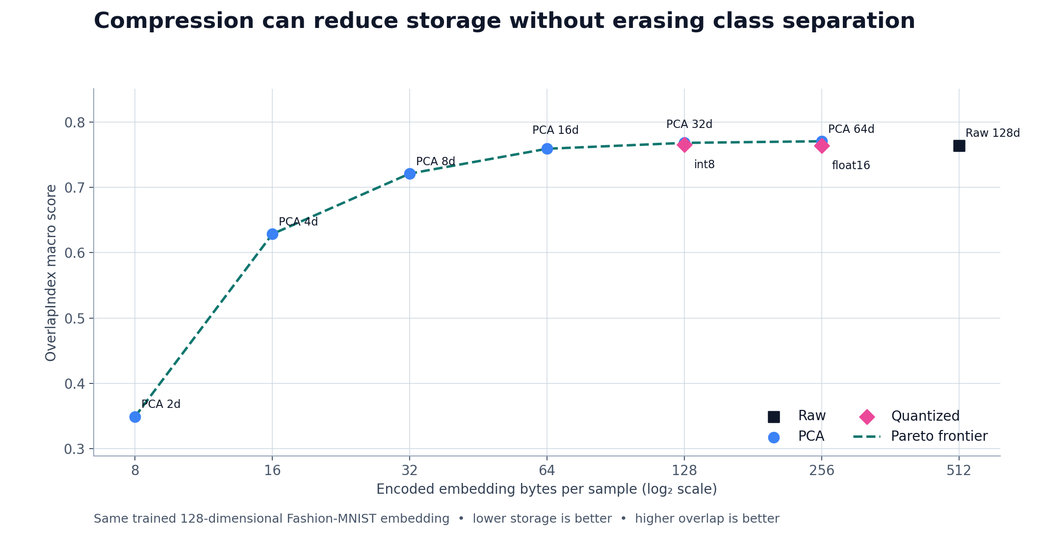
The network-free-after-download
fashion_mnist_visual_suite.py
also illustrates the storage-quality tradeoffs of PCA and quantization on a
trained penultimate embedding. Each point shows the measured OverlapIndex score
against encoded bytes per sample; the dashed line marks the non-dominated frontier.
from sklearn.decomposition import TruncatedSVD
from sklearn.feature_extraction.text import TfidfVectorizer
from sklearn.pipeline import Pipeline
from sklearn.preprocessing import Normalizer

from vertebrae import BenchmarkDataset, Evaluator, DatasetIdentity
from vertebrae.extractors import SklearnExtractor

pipeline = Pipeline(
    [
        ("tfidf", TfidfVectorizer(ngram_range=(1, 2), min_df=2)),
        ("svd", TruncatedSVD(n_components=128, random_state=42)),
        ("norm", Normalizer()),
    ]
)

dataset = BenchmarkDataset.from_arrays(texts, labels, modality="text", identity=DatasetIdentity.declared("example-dataset", "1"))
extractor = SklearnExtractor(
    name="tfidf_svd",
    pipeline=pipeline,
    # This manually versioned identity opts the fitted live pipeline into reuse.
    cache_identity="tfidf-svd-v1",
)

result = Evaluator(dataset=dataset, extractor=extractor).run()import numpy as np
import torch
from vertebrae import BenchmarkDataset, Evaluator, DatasetIdentity
from vertebrae.extractors import TorchExtractor
model = torch.load("/path/to/local_model.pt", map_location="cpu")
model.eval()
def collate_fn(batch):
return torch.as_tensor(np.asarray(batch), dtype=torch.float32)
def output_fn(raw_output):
return raw_output if isinstance(raw_output, torch.Tensor) else raw_output["embeddings"]
dataset = BenchmarkDataset.from_arrays(features, labels, modality="tabular", identity=DatasetIdentity.declared("example-dataset", "1"))
extractor = TorchExtractor(
name="local_torch",
model=model,
collate_fn=collate_fn,
output_fn=output_fn,
device="cpu",
checkpoint_paths=["/path/to/local_model.pt"],
cache_identity="local-torch-model-v1",
recipe_data={"checkpoint": "/path/to/local_model.pt"},
)
result = Evaluator(dataset=dataset, extractor=extractor).run()Torch extraction defaults to evaluation plus inference mode and restores the model's
prior state afterward. checkpoint_paths contributes provenance, but an already-loaded
live object still needs a maintained cache_identity for reusable caching.
One backbone may emit several named embeddings in a single evaluation. This is useful for comparing intermediate and final layers without duplicating extractor classes:
from vertebrae import Benchmark, CacheConfig
from vertebrae.extractors import HFVisionExtractor

benchmark = Benchmark(
    dataset,
    # The introductory remote model name below is intentionally unpinned.
    cache_config=CacheConfig(enabled=False),
)
benchmark.add_extractor(
    HFVisionExtractor(
        name="mnist_vit",
        model_id="farleyknight-org-username/vit-base-mnist",
        outputs=[
            {"name": "final_cls", "pooling": "cls"},
            {"name": "mid_cls", "pooling": "cls", "hidden_layer": 6},
        ],
        image_mode="rgb",
        batch_size=8,
    )
)

result = benchmark.run()
print(result.to_dataframe()[["extractor", "overlap_macro"]])
Each output is cached, compressed, scored, and reported independently. The complete extractor guide covers Hugging Face text, vision, audio, multimodal, time-series, and video adapters, as well as Keras, ONNX, sentence-transformers, timm, torchvision, OpenCLIP/SigLIP, TensorFlow Hub, JAX/Flax, tree, graph, and hosted embedding integrations.
from vertebrae import Benchmark

benchmark = Benchmark(dataset)
benchmark.add_extractor(tfidf_extractor)
benchmark.add_extractor(sentence_transformer_extractor)
benchmark.add_extractor(custom_extractor)

result = benchmark.run()
print(result.to_dataframe())
Named outputs can also be routed to different target or hierarchy views. See
hf_vision_mnist.py
for a complete layer comparison and
caltech101_vision_foundation_models.py
for a more realistic DINOv2/ViT workflow.
The examples below show how representation geometry can guide practical decisions: which layer to use, where a distribution shift first causes damage, whether a model learned a shortcut, and which backbone or downstream head to try next. Full protocols and result tables live in the linked guides and runnable scripts.
RepresentationMonitor repeatedly runs a fresh labeled Benchmark against live
extractors while your code retains control of training, cadence, checkpoints, and
optimization. Named outputs make it possible to inspect representation separation as
a function of both training progress and layer depth.
from vertebrae import (
    ConsoleReporter,
    EvaluationHistoryConfig,
    RepresentationMonitor,
)

monitor = RepresentationMonitor(
    fixed_probe_dataset,
    [live_torch_extractor],
    history_config=EvaluationHistoryConfig(
        storage="disk",
        path="representation-history.jsonl",
    ),
    reporters=[ConsoleReporter()],
)

for epoch in range(epochs):
    train_one_epoch(model)
    monitor.evaluate(epoch=epoch, metadata={"loss": training_loss})

history = monitor.history.to_dataframe()
Every call executes the configured benchmark stack and always recomputes embeddings,
even if an enabled cache is supplied. Use a fixed held-out probe dataset and control
evaluation cost through cadence, stability, and Separatix settings. The append-only
JSONL format supports protocol-validated resume and read-only loading. Restoring the
matching live model, optimizer, epoch, and step remains the caller's responsibility.
See the
representation monitoring guide and the network-free
examples/representation_monitoring.py Torch workflow.
The network-free-after-download
fashion_mnist_visual_suite.py
trains a compact two-block convolutional network and applies the same protocol
to real Fashion-MNIST evaluations. It carves a fixed, stratified validation set
out before training, leaves the official test set untouched, and disables
Separatix and stability repeats so each figure focuses on the raw OverlapIndex
diagnostic. For complementary visual examples of the underlying metrics, see the
OverlapIndex and
Separatix repositories.
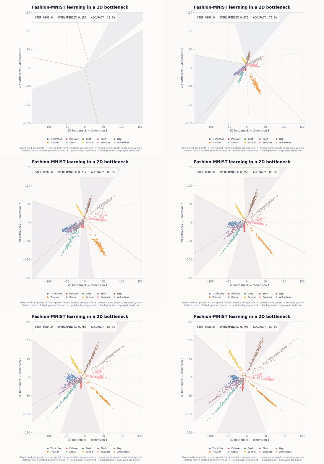
fashion_mnist_embedding_animation.py
trains a Fashion-MNIST classifier through a true two-dimensional bottleneck. The
points in the animation are the exact features consumed by the linear head—not a
PCA or UMAP projection—so the figure shows class geometry and validation accuracy
developing together on the same fixed, held-out examples.
The display aligns successive checkpoints to avoid distracting rotations without
changing the classifier's decisions. Frames labeled Display interpolation only
smooth the animation and are not trained model states; the accompanying CSV retains
the raw checkpoint metrics. In the checked-in run, the final bottleneck reaches raw
OverlapIndex 0.793 and 89.8% validation accuracy. Those values illustrate one
run rather than a general performance claim.
poetry install -E visuals
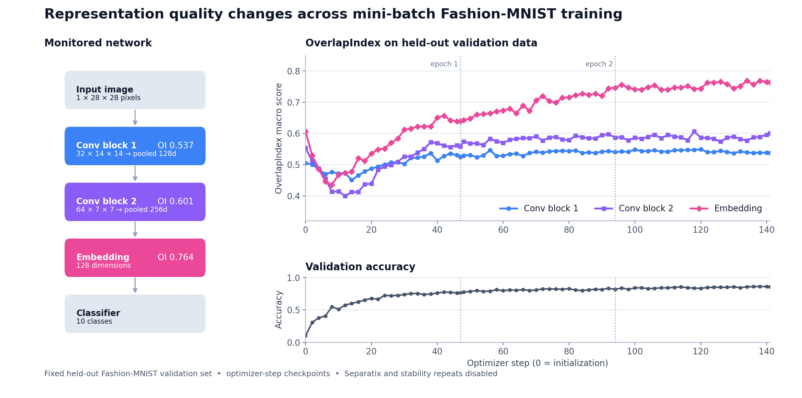
poetry run python examples/fashion_mnist_embedding_animation.pyTwo spatial convolutional representations and the learned 128-dimensional embedding are evaluated before training and every two optimizer steps over three epochs. The same layer identities and colors connect the network diagram to the monitoring curves. Fashion-MNIST's visually related apparel classes make it possible to compare how local features and the task-specific embedding evolve at different depths.
The companion
fashion_mnist_corruption_atlas.py
reuses the saved trained checkpoint and turns the untouched official test split into a
model-release probe. It evaluates clean images plus blur, Gaussian noise, occlusion,
contrast reduction, and rotation at four increasing severities without training another
model. A fixed k=5 makes OverlapIndex retention comparable across conditions within
each layer.
The atlas asks what failed, where did it start, and who was affected? It places within-layer OI retention beside accuracy and cross-entropy, then drills into affected classes and the first new pairwise confusions. Retention is contextual evidence, not a claim that classifier behavior improved.
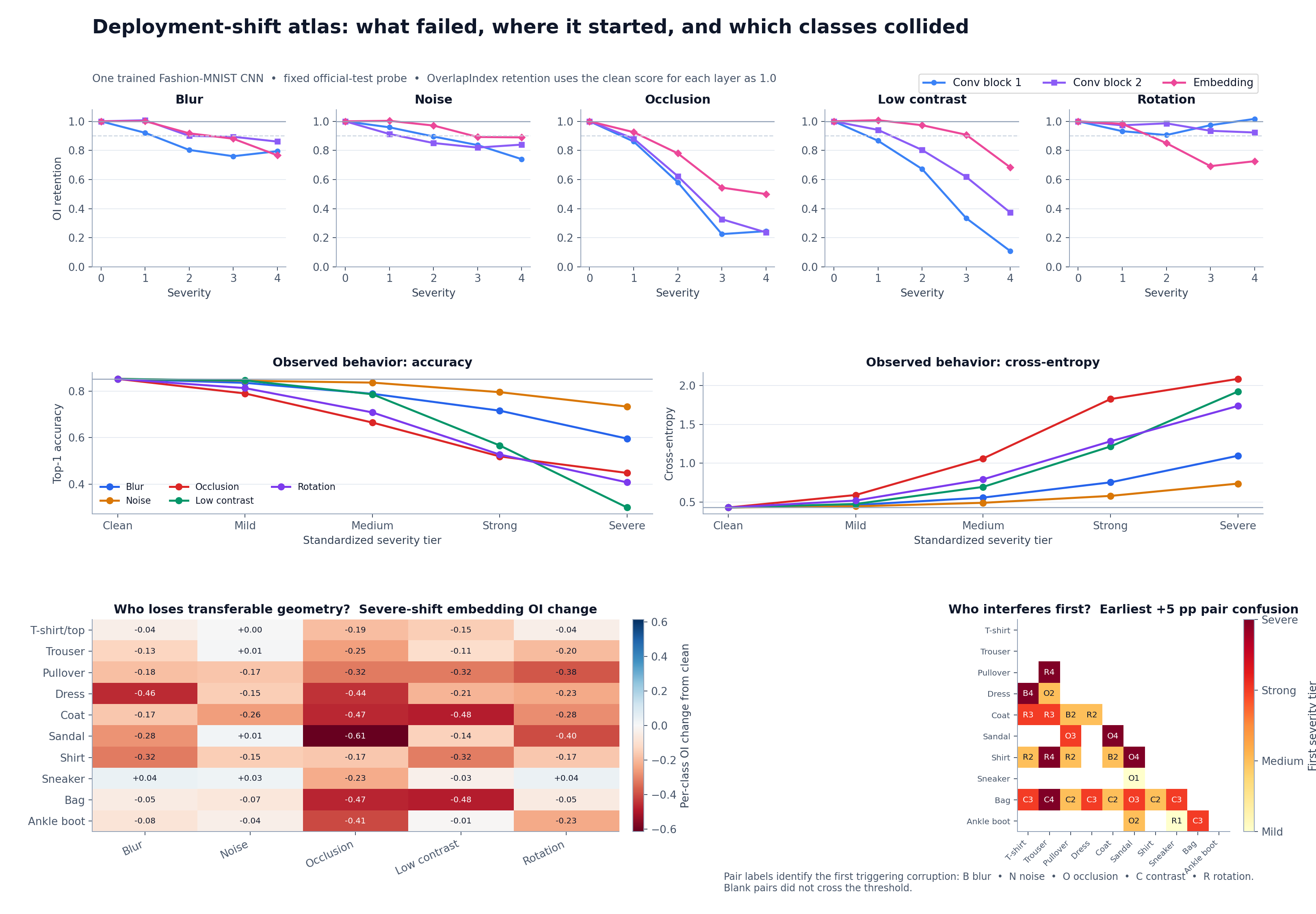
The run finds three distinct stories. Severe noise retains 0.89 of clean embedding
OI with accuracy 0.733. Severe contrast damages the backbone: first- and second-block
retention fall to 0.11 and 0.37, with accuracy 0.299. Rotation preserves early
features but damages the task representation: block 2 retains 0.92, the embedding
retains 0.73, and accuracy falls to 0.407. Those patterns suggest different fixes,
from preprocessing/backbone work for contrast to later-block fine-tuning for rotation.
The monitoring guide
retains the complete interpretation table, pair findings, production checklist, and
comparison caveats.
The companion
fashion_mnist_overfitting.py
trains clean-label and noisy-label CNNs from identical weights with identical images,
mini-batch order, optimizer settings, and schedules. Forty percent of a 1,000-example
training subset receives a deterministic wrong label. The models are then compared on
the same clean validation and corrupted-target probes, while held-out loss defines the
shaded overfitting region independently of OI.
The important story begins after the noisy model reaches its best validation loss.
From epochs 10 to 20, its final-embedding OI on the corrupted targets rises from 0.039
to 0.313, while the clean control remains near zero on those arbitrary labels. At the
same time, the noisy model's clean-probe OI stalls near 0.63, while the control
continues from 0.669 to 0.718. The noisy model is not merely fitting the wrong
answers at its output. Its late representation is increasingly reorganizing around
those answers while making no further progress on transferable garment structure.
The layer comparison localizes that tradeoff. Early features remain similar, the second block begins to diverge, and the strongest arbitrary-target geometry appears in the final embedding. For a practitioner, that pattern argues against discarding the entire backbone. It points instead toward restoring an earlier checkpoint, preserving the reusable early features, auditing the corrupted labels, and focusing regularized or noise-robust retraining on the later representation stages.
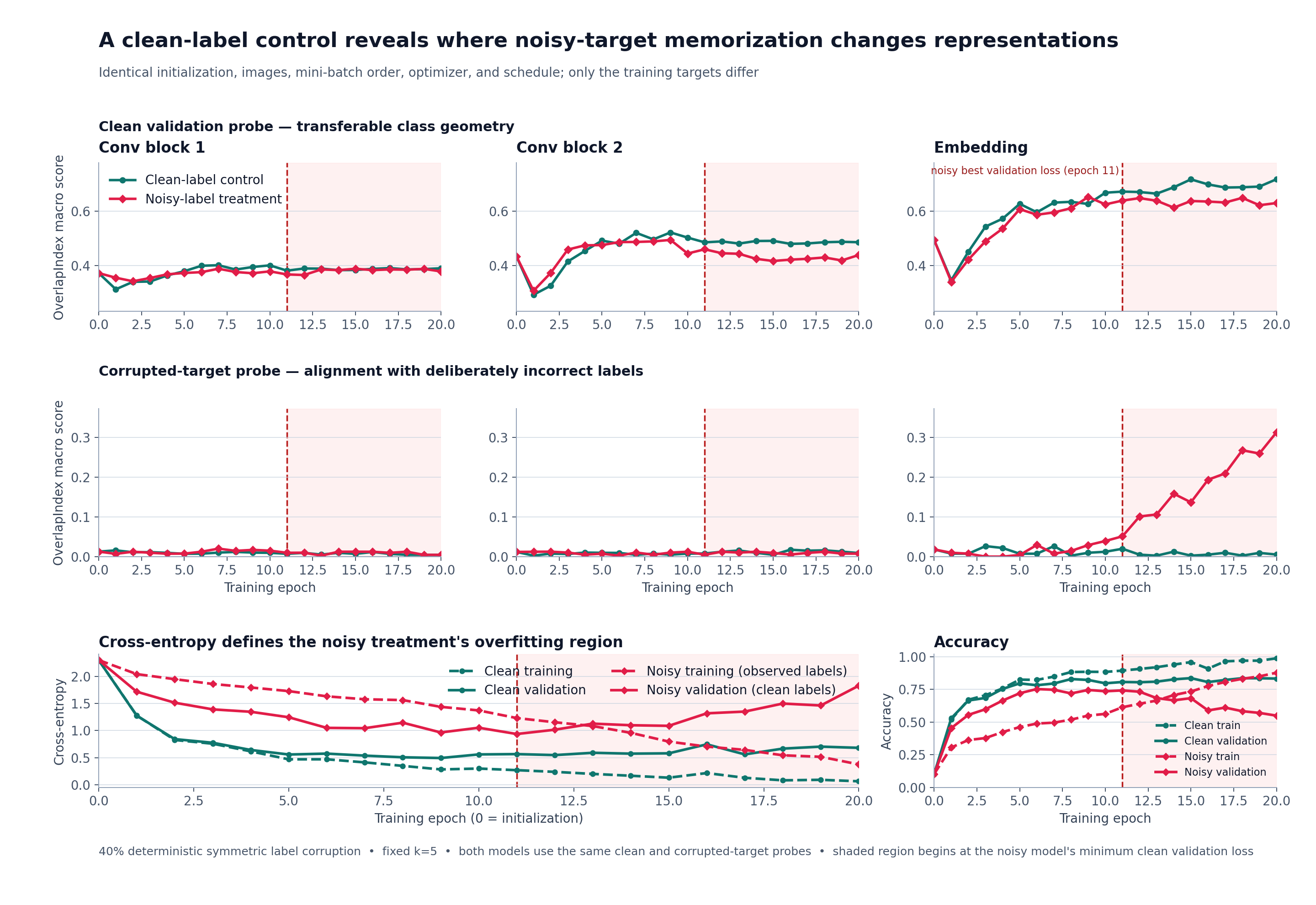
OI is not an overfitting detector by itself. Held-out loss establishes the failure; OverlapIndex reveals what geometry the model learned and where that learning entered the representation hierarchy. The full monitoring case study preserves the control design, interpretation table, and practical response patterns.
A model can look excellent on its headline metric while organizing its representation
around the wrong semantics. The
colored_fashion_mnist_shortcut.py
experiment demonstrates how named target views, a controlled reference run, and an
external behavioral intervention can expose that failure mode.
The practical question is deliberately simple: if garment color predicts garment class during training, does a CNN learn the garment or the color shortcut? Accuracy alone cannot answer this on the training distribution. Likewise, high class OI alone cannot answer it if class and color are correlated in the representation probe. The experiment therefore separates three jobs:
- A paired control isolates the effect of the class-color correlation.
- A decorrelated audit probe asks what each layer organizes.
- Counterfactual recoloring asks whether the learned organization changes behavior.
Two identically initialized CNNs receive the same 2,000 garments, targets, batches, and 12-epoch schedule. Color is useless in the control but predicts class 85% of the time in the treatment. A held-out 2,000-garment probe is rendered grayscale, canonical, independently colored, and with a reversed mapping.
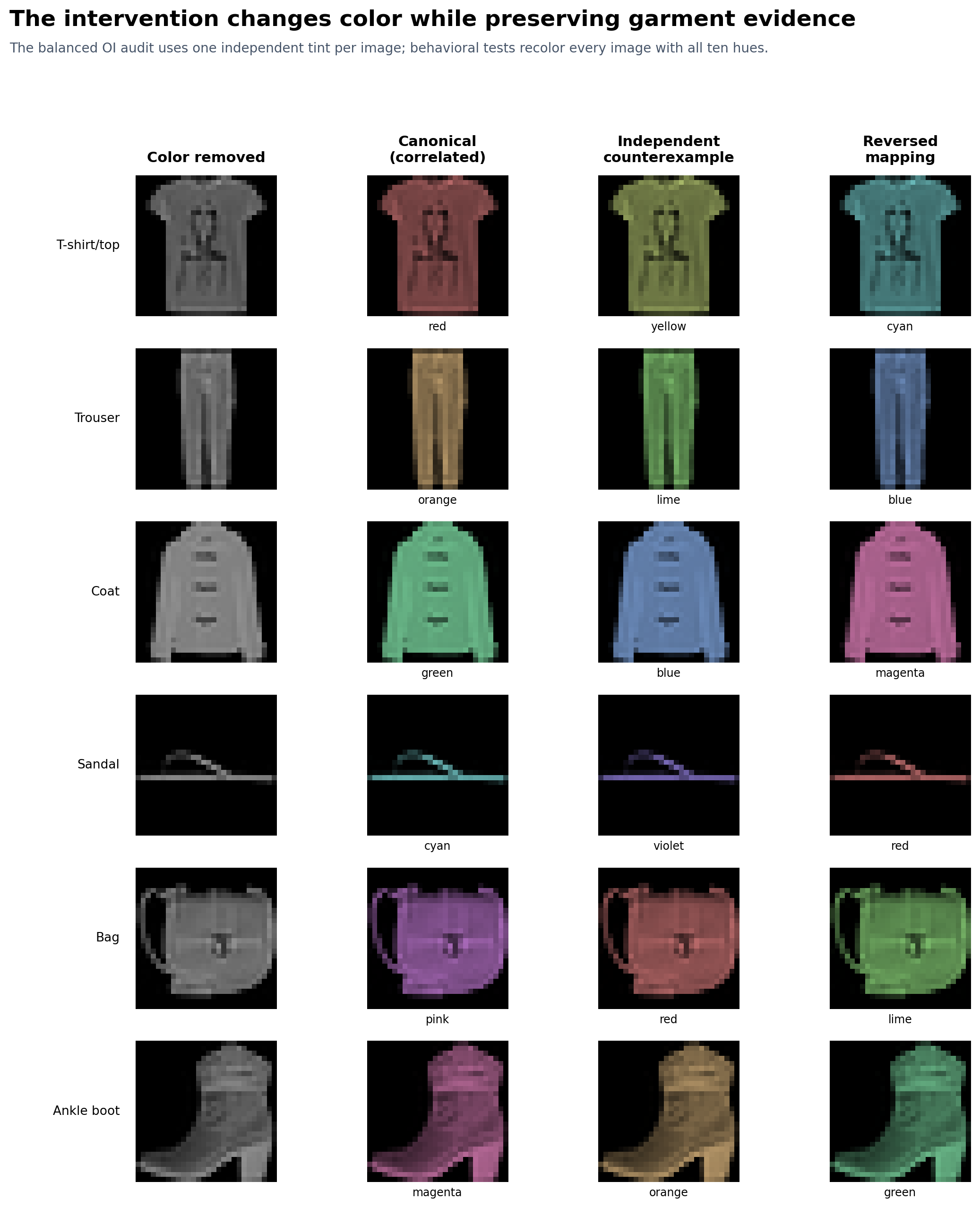
The representation audit balances class×color cells and registers two views:
intended_class: the garment category that the classifier should learn;nuisance_color: the tint that should not determine the prediction.
Balancing keeps garment and color statistically independent so the views describe distinct geometry. Five paired seeds measure variation across trained models.
The treatment appears better in-distribution at 91.42% versus 82.63%, but trails the
control by 13.81 points on balanced colors and 35.54 points under reversal.
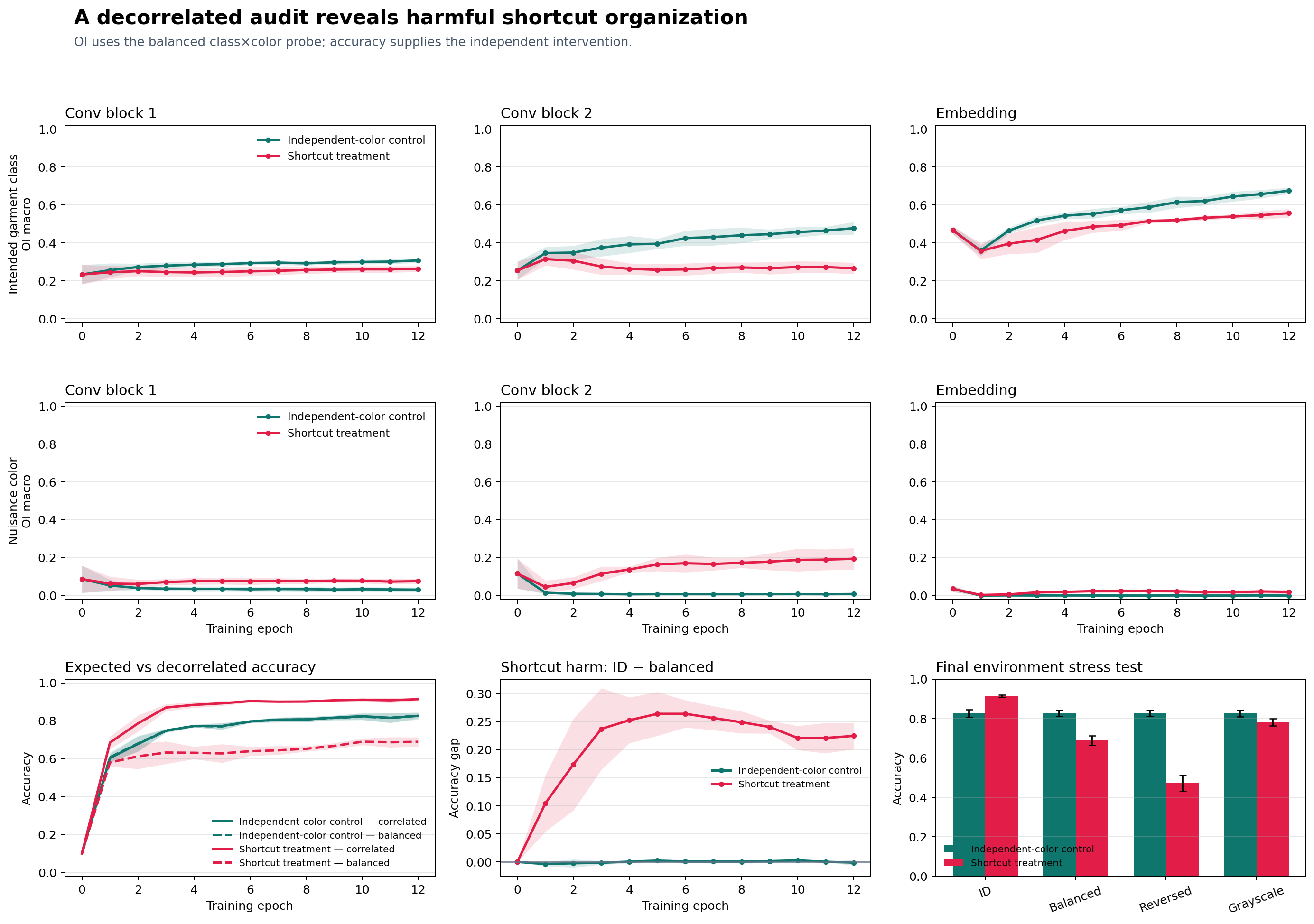
At epoch 12, the control's final embedding reaches intended-class OI 0.675, versus
0.557 for the treatment. In block 2, nuisance-color OI is 0.009 for the control and
0.194 for the treatment. The paired effect localizes shortcut structure before the
classifier head.
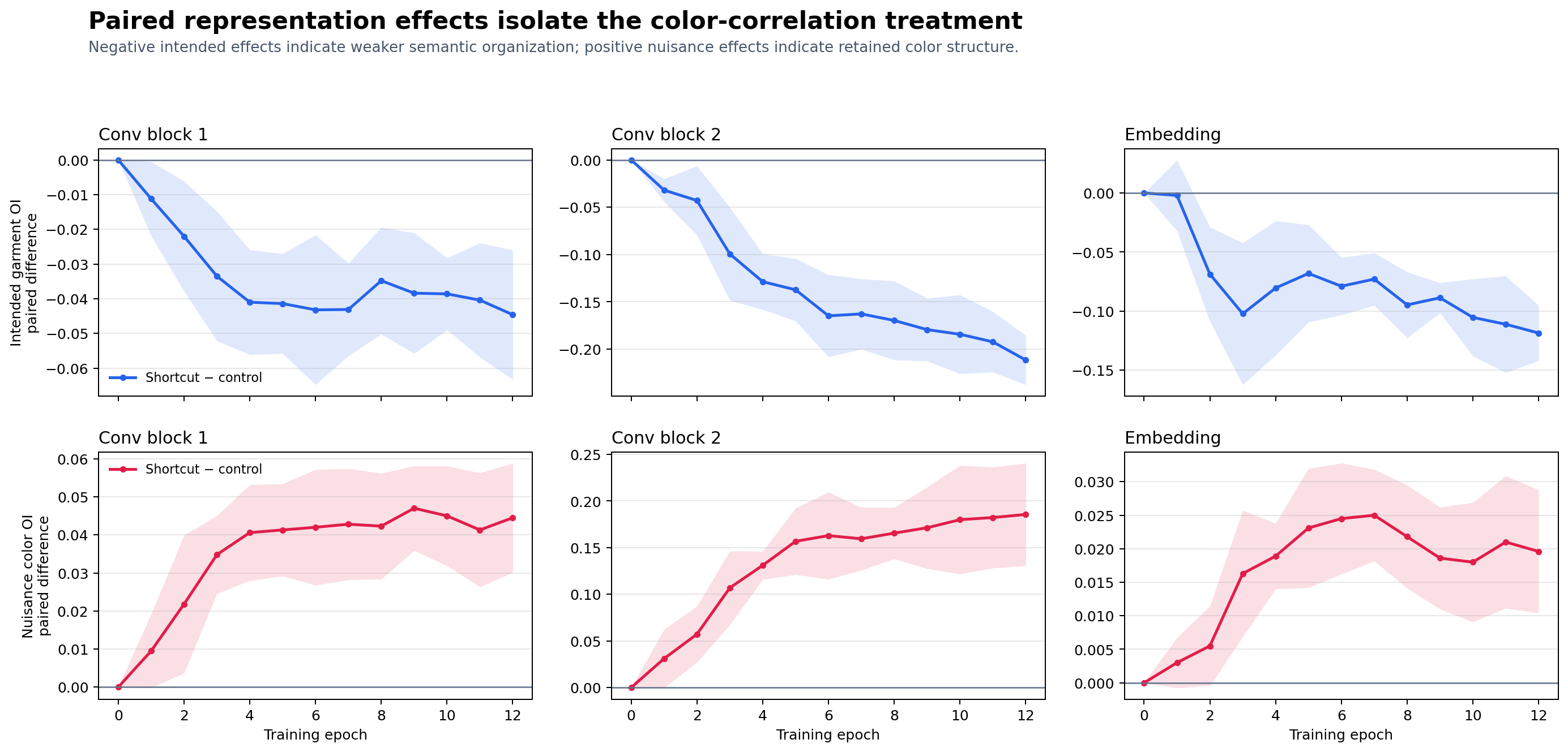
Final-embedding color OI can remain low while predictions are color-sensitive: a classifier may exploit a weak or class-conditional direction without producing ten globally separated color clusters. OI localizes geometry; counterfactual accuracy tests whether the nuisance affects decisions.
Across all ten recolorings, treatment accuracy falls to 68.28% versus 82.70% for
the control. Prediction changes under recoloring rise from 3.42% to 62.17%, and
the treatment's 10th-percentile class×color accuracy is only 6.75%. Aggregate
in-distribution accuracy had hidden nearly unusable garment-color cells.
The transferable pattern is to name intended and nuisance targets, decorrelate them on a fixed probe, compare with a controlled reference, monitor the same layers, intervene on the nuisance, and repeat paired training seeds. The full shortcut case study retains the complete result tables, audit checklist, caveats, and reproduction command.
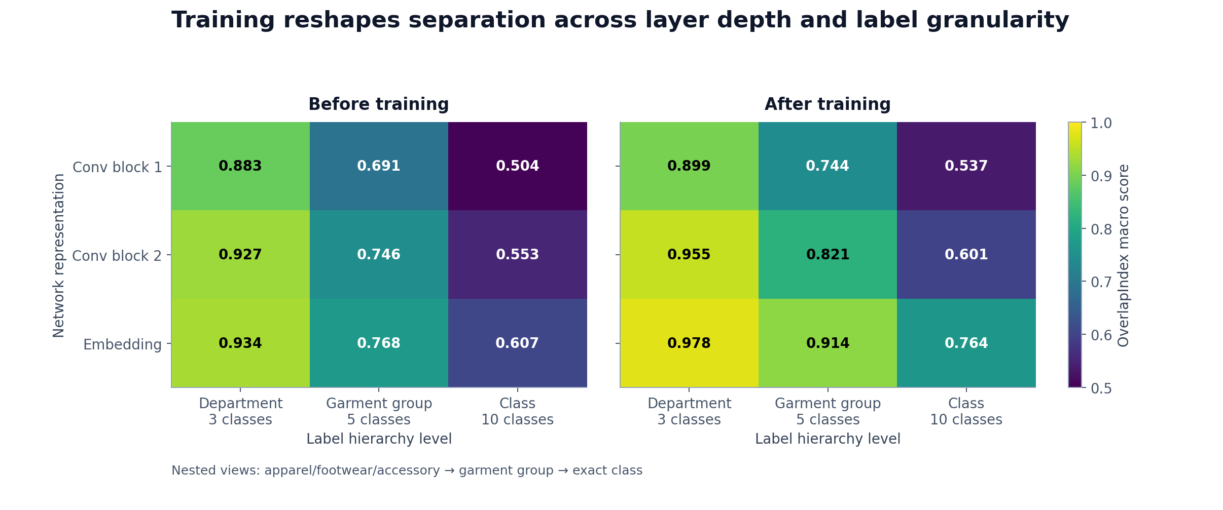
The same representations are evaluated against nested department, garment-group, and exact-class label views before and after training.
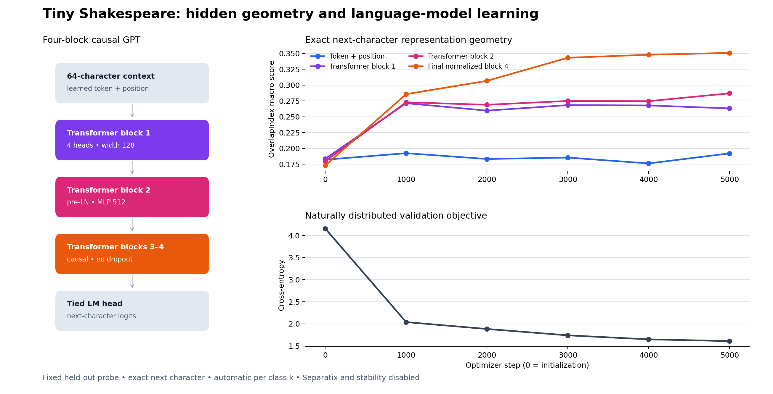
tiny_shakespeare_transformer_visual_suite.py
extends the same monitoring pattern to a character GPT. It tracks named hidden states
against a fixed next-character probe while language-model loss and accuracy remain
separate behavioral measures. In the checked 5,000-step run, validation cross-entropy
falls from 4.1555 to 1.6097 while final-block macro OverlapIndex rises from 0.173
to 0.351, localizing most of the learned target geometry to the transformer blocks.
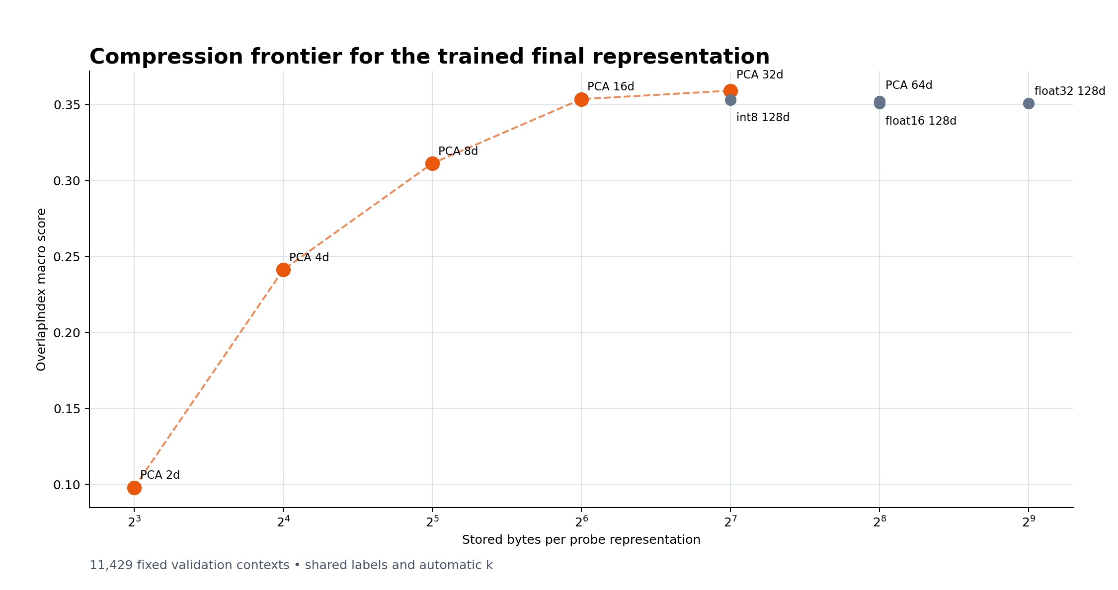
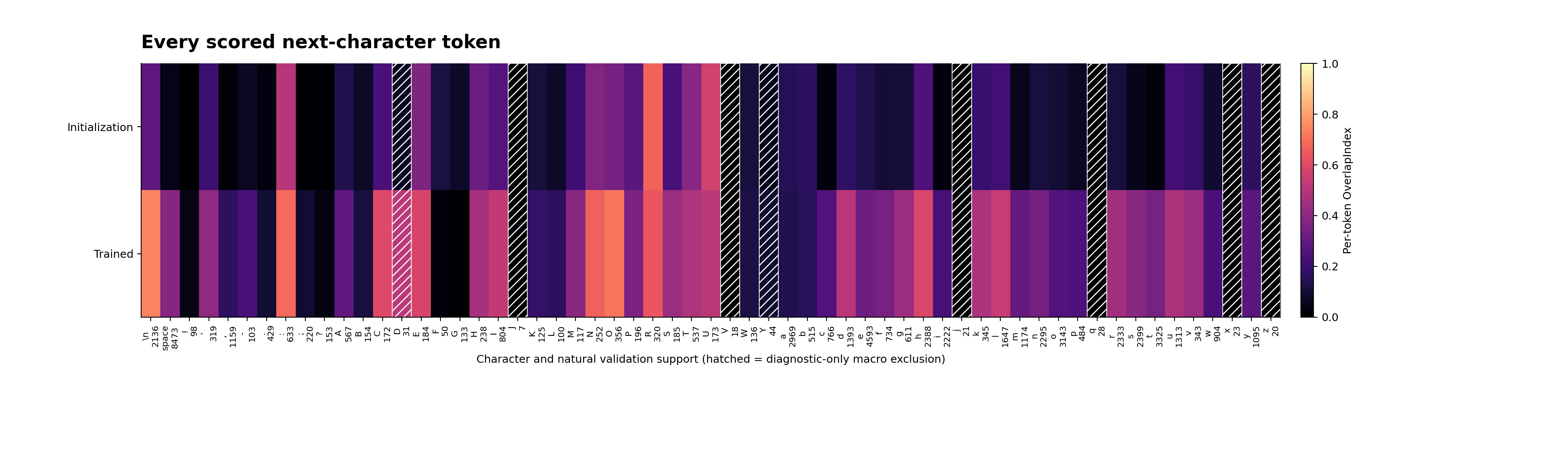
The monitoring guide contains the full data split, support rules, compression results, and reproduction profiles.
Reproduce these monitoring examples with:
poetry install -E visuals
poetry run python examples/fashion_mnist_visual_suite.py
poetry run python examples/fashion_mnist_embedding_animation.py
poetry run python examples/fashion_mnist_corruption_atlas.py
poetry run python examples/fashion_mnist_overfitting.py
poetry run python examples/colored_fashion_mnist_shortcut.py --repeats 5
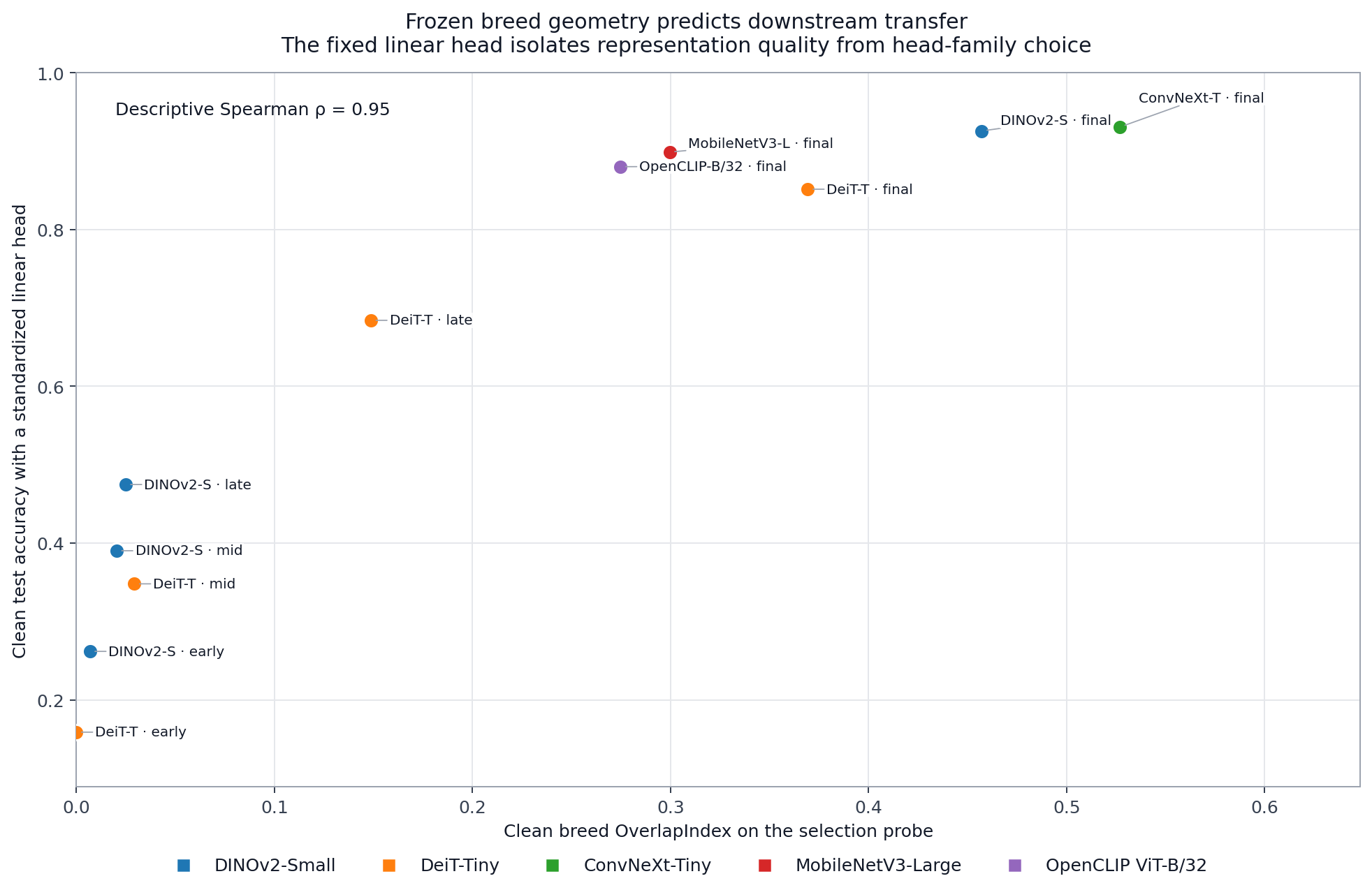
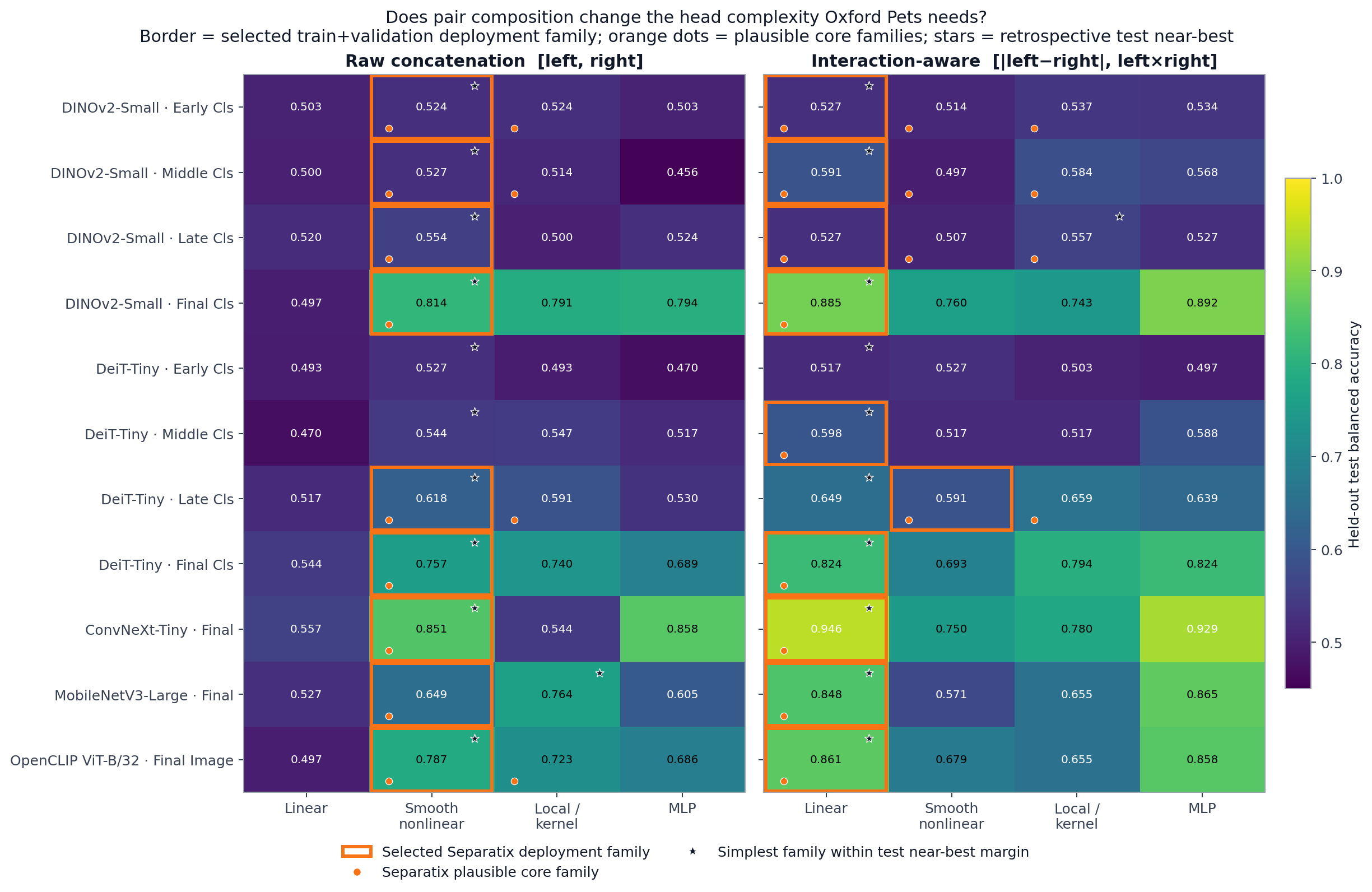
poetry run python examples/tiny_shakespeare_transformer_visual_suite.pyoxford_pets_backbone_selection.py
shows the two decisions separately: use OverlapIndex to shortlist frozen backbone
outputs, then use Separatix to decide which downstream family is worth testing. On
Oxford-IIIT Pet, the representation ranking tracks held-out transfer quality while the
head guidance distinguishes genuinely nonlinear structure from a relationship that can
be made linear with better features.
The second plot shows the practical payoff: exposing difference and product features can turn an apparently nonlinear comparison into one that a simple linear head handles well. Try a clearer task representation before automatically paying for a larger head.
poetry install -E backbone-selection
poetry run python examples/oxford_pets_backbone_selection.pyfood101_nonlinear_backbone_bridge.py is
the runnable example behind the opening story. It compares a linear probe with
OverlapIndex while fixed linear, quadratic, kNN, and RBF heads provide independent
downstream checks. The useful pattern is simple: the methods agree on easy linear
geometry, but OverlapIndex is better able to surface useful nonlinear organization.
The nuisance control is a reminder to validate the shortlisted model on the real task.
See the scoring guide for the full methodology and results.
poetry install -E backbone-selection
poetry run python examples/food101_nonlinear_backbone_bridge.py
poetry run python examples/plot_food101_overlap_vs_linear_probe_story.pyfood101_selector_runtime_scaling.py
compares the cost of scoring the same frozen embeddings. A linear probe is faster on
the smallest panel; OverlapIndex catches up as the dataset grows and reaches a 2×
median speedup at 25,600 embeddings in this Food-101 run.

The crossover depends on hardware, feature dimension, class count, and implementation, so benchmark on your own embeddings when runtime matters. The script and tracked summary make that easy.
poetry run python examples/food101_selector_runtime_scaling.py --output-dir examples/output
poetry run python examples/plot_food101_selector_runtime_scaling.pyRetrievalBenchmark evaluates frozen query embeddings against an explicit gallery
and graded relevance judgments. It is an exact, training-free ranking protocol and
is separate from ordinary labeled OverlapIndex benchmarking.
from vertebrae import RetrievalBenchmark, RetrievalConfig, RetrievalDataset, DatasetIdentity
from vertebrae.extractors import PrecomputedExtractor

dataset = RetrievalDataset.from_embeddings(
    query_embeddings,
    gallery_embeddings,
    relevance=[("query-1", "document-9", 2.0)],
    query_ids=["query-1"],
    gallery_ids=["document-9"],
    identity=DatasetIdentity.declared("example-dataset", "1"),
)

result = RetrievalBenchmark(
    dataset,
    [PrecomputedExtractor("candidate")],
    retrieval_config=RetrievalConfig(primary_metric="ndcg@10"),
).run()
Relevance can be a NumPy/scipy query-by-gallery matrix or sparse
(query_id, gallery_id, grade) records. Nested Python lists are records; construct
nested-list matrices explicitly with RetrievalDataset.from_relevance_matrix(...).
Every query must retain an eligible positive after exclusions. Reports include NDCG, precision, recall,
hit rate, MRR, mAP, and similarity diagnostics. See
the retrieval guide for branch-aware extractors,
bidirectional scoring, exclusions, compression, and artifact workflows.
For contrastive extractors with independently encodable sample and text branches,
ZeroShotBenchmark evaluates whether fixed class prompts address the dataset in the
model's shared embedding space. It trains no head and requires explicit prompts. The
zero-shot rank and ordinary sample-embedding overlap are reported side by side; they
are not combined into a universal backbone score. See docs/zero_shot.md and the
network-free examples/zero_shot_callable.py workflow.
The OpenCLIP CIFAR-10 experiment in
examples/zero_shot_transfer_structure.py separates sample structure from text
alignment. It encodes a balanced set of 500 images exactly once with the frozen
OpenCLIP image encoder, producing one fixed image-embedding matrix. OverlapIndex is
then calculated once from that matrix and the CIFAR-10 labels.
The same image matrix is reused with three explicit prompt protocols. Only the text
changes: cat, a photo of a cat, or
a low-resolution CIFAR-10 image of a cat, for example. Each string passes
through the same frozen text encoder and produces a different class prototype. Model
weights, image embeddings, and the shared embedding space remain unchanged; only the
prototype locations used for cosine-similarity classification move.
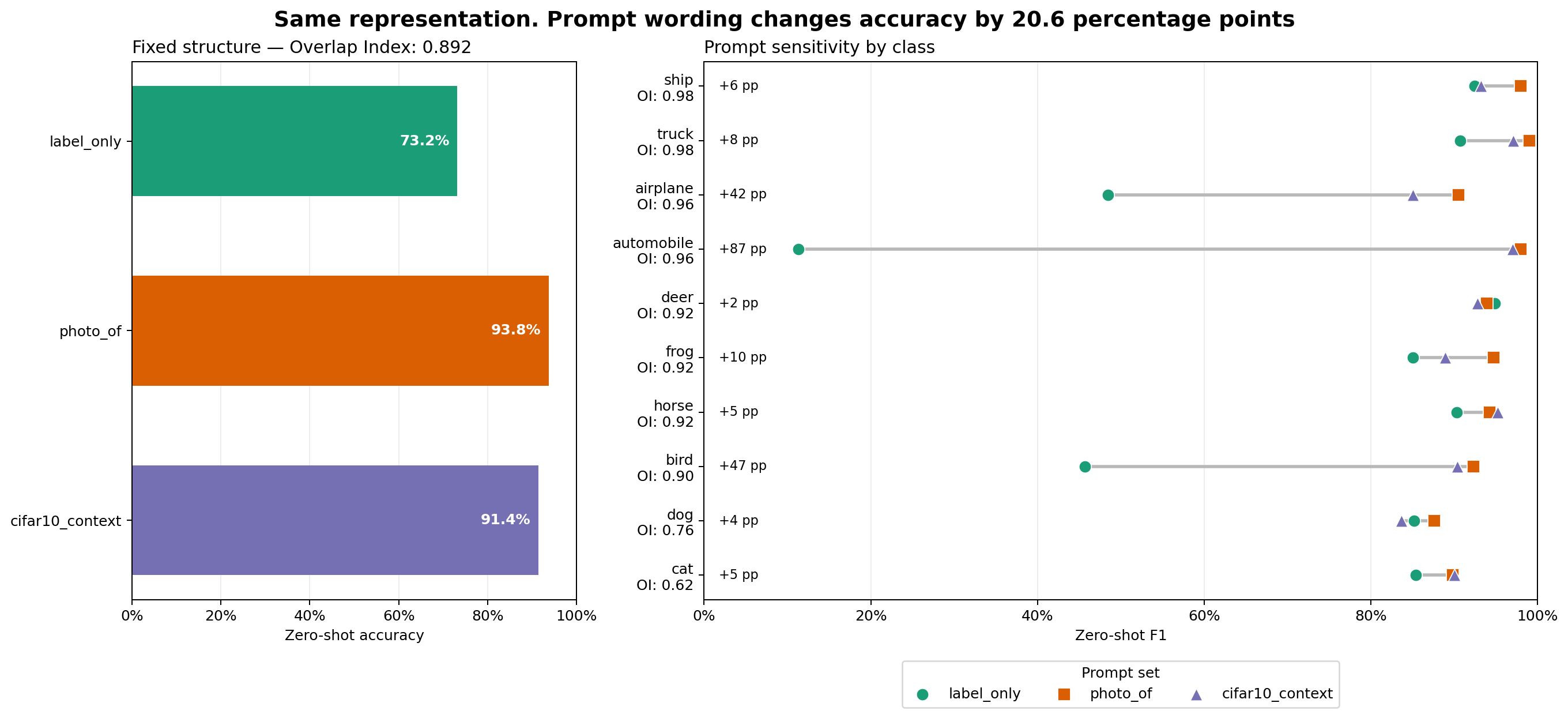
The left panel shows the central result. The sample representation has a fixed macro
OverlapIndex of 0.892, while zero-shot accuracy changes from 73.2% with bare labels
to 93.8% with photo prompts, a 20.6 percentage-point improvement without changing
the image representation. Weak initial zero-shot accuracy therefore did not imply weak
transfer features in this run; the original text prototypes addressed otherwise strong
image structure poorly.
The right panel shows the same distinction per class. Rows are ordered by their fixed
per-class OverlapIndex. Colored markers are zero-shot F1 under each prompt protocol,
the gray segment is the prompt-driven F1 range, and the percentage-point annotation
quantifies prompt sensitivity. automobile, for example, has strong structure
(OI: 0.96) but an 87-point F1 range across prompts. Per-class OverlapIndex and F1
should not be compared as interchangeable values: they answer different questions
despite both being bounded scores.
For practitioners, the two signals suggest different next actions:
| sample structure | zero-shot alignment | practical next step |
|---|---|---|
| strong | weak or prompt-sensitive | Keep the backbone; improve class wording, use a predeclared prompt ensemble, or train a supervised head. |
| strong | strong and stable | The frozen representation is both transferable and naturally text-addressable for this protocol. |
| weak | strong | Zero-shot classification works, but inspect whether the feature geometry is robust enough for broader transfer. |
| weak | weak | Investigate another backbone, domain adaptation, or a different data representation. |
Prompt alternatives should be declared before evaluation or chosen on a separate validation set. Trying many prompts against test labels and reporting only the winner turns prompt design into test-set tuning. The experiment is intentionally diagnostic: it does not combine OverlapIndex and zero-shot accuracy into one model-quality score.
Use ZeroShotCandidate(extractor, sample_branch, text_branch) when compared models
use different branch names. OpenCLIP keeps its image-only ordinary default while its
native text_branch remains available for zero-shot. Callable adapters cache only
when their functions have portable paths or an explicit cache_identity.
Retrieval and zero-shot compression keep both sides in one representation space.
Learned retrieval transforms are fitted on the gallery and applied to queries;
learned zero-shot transforms are fitted on samples and applied to prompt embeddings.
The CLI exposes these paired workflows through compress-retrieval and
compress-zero-shot.
Every benchmark always records the built-in overlap metric. You can score the
same full embedding batch with additional metrics and choose one as the ranking
criterion. A custom metric returns a finite aggregate score and may include
JSON-safe diagnostics, warnings, and metadata.
For protocol parity, categorical labels and groups passed to custom metrics are
marked semantic-key strings locally and on distributed workers; regression targets
remain numeric. Read original typed provenance and display values from
target_metadata["label_catalog"] when needed.
from vertebrae import Benchmark, CallableMetric

def domain_margin(embeddings, labels, *, groups=None, seed=None):
    return {"score": 0.87, "diagnostics": {"rule": "domain margin"}}

result = Benchmark(
    dataset,
    [extractor],
    metrics=[CallableMetric("domain_margin", domain_margin)],
    primary_metric="domain_margin",
).run()
The overlap result remains available in every ExtractorResult and continues
to drive stability and Separatix. For artifact or CLI workflows, use an
importable callable path such as my_project.metrics:domain_margin; see
the scoring guide
and the distributed-readiness guide.
Dense segmentation evaluation scores spatial feature cells after they are aligned to semantic mask labels. It measures representation organization for retained tokens; it is not an IoU, mask-accuracy, or boundary-quality metric.
Both dense spatial outputs and other structured model outputs become ordinary labeled embedding rows before scoring:
flowchart TB
    spatial_source["Spatial path<br/>image, semantic mask, declared feature grid"] --> spatial_align["Assign cells by mask coverage<br/>filter ambiguity and sample deterministically"]
    structured_source["Structured path<br/>parent sample, unit annotations, emitted rows"] --> structured_align["Select and align emitted rows<br/>to declared unit annotations"]

    spatial_align --> rows["Materialized BenchmarkDataset rows<br/>embeddings, targets, parent groups, provenance"]
    structured_align --> rows
    rows --> scoring["Standard labeled-embedding scoring<br/>OverlapIndex, stability, gated Separatix"]
from vertebrae import (
    Benchmark,
    CallableSpatialExtractor,
    SegmentationConfig,
    SegmentationDataset,
    SpatialLayout,
    SpatialOutputSpec,
)

dataset = SegmentationDataset.from_arrays(
    images=images,
    semantic_masks=masks,
    identity=DatasetIdentity.declared("example-dataset", "1"),
)

extractor = CallableSpatialExtractor(
    "encoder",
    transform_fn=extract_spatial_features,
    output_specs=[
        SpatialOutputSpec(
            name="stage_4",
            layout=SpatialLayout(grid_height=14, grid_width=14),
        )
    ],
)

result = Benchmark(
    dataset=dataset,
    extractors=[extractor],
    segmentation_config=SegmentationConfig(max_tokens_per_class=10_000),
).run()
See docs/segmentation.md for background handling, ambiguity filtering,
instance caps, grouped diagnostics, and precomputed segmentation embeddings.
Structured extractors flatten one declared per-parent unit matrix into a grouped embedding dataset, preserving unit provenance and parent groups. This supports representation diagnostics for regions, tokens, frames, keypoints, depth cells, and latent slots. It does not substitute task-native metrics such as mAP, IoU, WER/CER, OKS, depth error, or reconstruction quality.
Unit annotations may use single-label, multi-label, or one-/multi-target
regression targets, provided every parent uses the same resolved schema. Local
unit IDs may repeat across parents; materialization generates parent-aware
global IDs and retains the supplied value as local_unit_id in provenance.
Dense and scipy sparse per-parent matrices are supported without premature
densification.
from vertebrae import Benchmark, BenchmarkDataset, UnitAnnotation, DatasetIdentity
from vertebrae.extractors import CallableStructuredExtractor, StructuredOutputSpec

dataset = BenchmarkDataset.from_arrays(X=pages, y=document_labels, modality="image", identity=DatasetIdentity.declared("example-dataset", "1"))
dataset = dataset.with_unit_annotations(
    [
        UnitAnnotation(labels=["heading", "body"]),
        UnitAnnotation(labels=["heading", "body"]),
    ],
    unit_type="document_region",
)

extractor = CallableStructuredExtractor(
    name="layout_encoder",
    transform_fn=extract_region_embeddings,  # one 2D matrix per page
    output_specs=[StructuredOutputSpec(name="regions", unit_type="document_region")],
)
result = Benchmark(dataset, [extractor]).run()
When the model emits unmatched rows (for example special tokens or sampled
frames), supply an explicit alignment rule such as
drop_special_rows(leading=1) or select_frame_rows(...). Typed adapters are
also available for detection/layout, sequence labeling, keypoints, depth, and
latent slots. See
the dataset guide
and the extractor guide,
alongside the runnable
examples/structured_*.py workflows.
The package covers labeled classification, multi-label, regression, named target and hierarchy views, structured units, dense segmentation, exact retrieval, fixed-prompt zero-shot alignment, monitoring, compression, custom metrics, local/distributed execution, and local/S3/GCS artifacts. SciPy sparse matrices and arrays remain sparse through classification, multi-label, regression, and stability scoring, and at the vertebrae boundary when passed into Separatix; multi-label targets may also be sparse binary indicators. The complete workflow inventory groups every supported dataset, extractor, protocol, report, and CLI stage. The distributed guide documents trusted pickle inputs, cache identity, immutable manifests, streaming contracts, Ray/Dask/SLURM execution, and cloud-store requirements.
Resource profiling can be enabled when deployment cost is part of representation selection:
from vertebrae import ResourceProfilingConfig

result = Benchmark(
    dataset,
    extractors=[small_backbone, large_backbone],
    resource_profiling_config=ResourceProfilingConfig(enabled=True),
).run()

print(result.to_dataframe())
print([item.name for item in result.quality_cohort()])
The profile observes the benchmark's real local extraction calls. It reports
first-call and warm latency, observed throughput, host memory, supported device/model
footprints, and logical raw/compressed embedding storage. It does not change quality
ranking. A cache hit remains a cache hit and reports inference as unmeasured; use
CacheConfig(force_recompute=True) when a fresh inference measurement is required.
Profiles distinguish complete, partial, unavailable, and CPU-not-applicable evidence. Latency remains meaningful only with its batch, device, precision, synchronization, and cache context; it is a workload observation rather than a hardware-normalized score. The results guide documents native device adapters and distributed endpoint profiles.
Each benchmark run returns structured results that include:
- dataset summary,
- extractor summary and recipe metadata,
- overlap scores plus per-class, per-label, or per-target diagnostics,
- Separatix recommendation, confidence, and report details when the overlap gate passes,
- label-view, target-view, segmentation, structured-unit, grouping, and target-type metadata when present,
- every configured metric result and the selected primary ranking metric,
- compression metadata and compressed dimensions,
- stability summaries,
- warnings and recommendations,
- reproducibility metadata.
Only results whose selected metric declares aggregate_valid=True participate in
rankings, quality cohorts, top recommendations, or resource comparisons. When no
valid aggregate remains, reports say that ranking is unavailable instead of promoting
an invalid result.
Results can be rendered directly to Markdown or JSON:
result.save_json("result.json")
result.save_markdown("report.md")
You can also convert rankings into a DataFrame with result.to_dataframe().
Compression-aware results include the compression method and compressed dimension, and quantized runs preserve calibration metadata in the structured result payload.
Separatix is stored as the default classifier-complexity report field. JSON output preserves the full Separatix report. Markdown and DataFrame views surface the main recommendation, confidence, and compact explanation fields that are usually the most actionable.
Separatix 0.1.1 adds an uncertainty-aware family frontier to those summaries.
SeparatixResult.family_guidance reports the minimum recommended family,
plausible alternatives, the decision method, selected family/probe and recipe id,
MLP-override status, and paired-comparison status/method. The normalized probe
evaluation context records estimator alignment, the CV/cohort plan, and effective
train size. Use SeparatixResult.probe_recipe(...) or
selected_probe_recipe() with Separatix's make_probe_estimator(...) factory to
reproduce the exact diagnostic estimator. A missing recipe is reported as
unavailable rather than replaced with a hand-built approximation.
When MLP probes are enabled, their compute trigger is separate from the paired
improvement required to override a simpler family; an untriggered MLP is therefore
not evidence that linear guidance won an exhaustive comparison.
Separatix is also the source of probe-style summary fields, so vertebrae does not fit a second probe system alongside the complexity diagnostic.
The key component of the report is the performance and comparison table. The
following is the current output generated by
examples/sklearn_wine_pipeline.py.
| rank | extractor | primary_metric | primary_score | overlap_macro | stability_interval | weakest_class | best_probe | probe_metric | probe_score | embedding_dim | recommendation |
|---|---|---|---|---|---|---|---|---|---|---|---|
| 1 | wine_standard_scaler_all_features | overlap | 0.9232 | 0.9232 | 0.9058-0.9279 | class_1 | linear | balanced_accuracy | 0.9812 | 13 | strong_candidate |
| 2 | wine_standard_scaler_pca_6 | overlap | 0.9179 | 0.9179 | 0.9051-0.9368 | class_1 | kernel_approx | balanced_accuracy | 0.9767 | 6 | strong_candidate |
| 3 | wine_minmax_pca_2 | overlap | 0.9079 | 0.9079 | 0.9366-0.9455 | class_1 | smooth_poly | balanced_accuracy | 0.9756 | 2 | strong_candidate |
| 4 | wine_quantile_pca_1 | overlap | 0.4554 | 0.4554 | 0.3455-0.4554 | class_2 | 1 | poor_frozen_representation_weak_class_attention |
The full generated table also includes target_view, label_view,
overlap_score, overlap_weighted, compression fields, and Separatix fields.
The compact table above keeps the README readable while preserving the values used
for the ranking. Its recommendation column is Vertebrae's representation-quality
summary; the separate separatix_recommendation column uses the eight canonical
Separatix labels described below.
By default, extractors are ranked by overlap. When a custom primary_metric is
configured, they are ranked by that metric instead; the overlap columns remain
available for representation diagnostics and Separatix gating.
For classification and multi-label targets, discrete OverlapIndex scores are
bounded to [0, 1]: 1.0 indicates perfect class separation and 0.0 indicates
perfect class overlap. The discrete score is not permutation-null calibrated, so
0.5 has no special null interpretation. ContinuousOverlapIndex uses the separate
regression calibration described in the scoring documentation.
The easiest way to interpret the report is:
- Start with
primary_metricandprimary_score. By default these are overlap; with a custom metric they identify the configured ranking signal. - Inspect
overlap_macroand per-class overlap scores as the standard vertebrae representation diagnostic, even when another metric ranks the candidates. - Use the vertebrae
recommendationfield as a quick summary of representation quality under the benchmark protocol. - Use
separatix_recommendationandseparatix_confidenceto understand what kind of downstream classifier complexity the labeled embedding seems to imply once the representation is already reasonably separated. The recommendation uses exactly eight canonical labels shared across target modes:linear_likely_sufficient,smooth_nonlinear_recommended,kernel_or_local_recommended,high_capacity_or_partitioning_recommended,feedforward_mlp_recommended,feature_or_target_bottleneck_likely,insufficient_data_or_unreliable_geometry, andinconclusive. - When Separatix columns are blank, the diagnostic was disabled, did not clear the overlap gate, or did not return that field. Check the per-extractor skip reason before interpreting the blank.
- Treat
best_probe,probe_metric, andprobe_scoreas Separatix-derived quick-check columns. They are blank when Separatix is disabled, skipped, or does not report a baseline probe score. The metric is target-aware rather than always being accuracy. - Use the family frontier to plan downstream experiments: start with
minimum_recommended_family, retainplausible_familiesas unresolved alternatives, and inspect paired evidence and effective train size before calling a recommendation a mismatch. The shared machine-readable label does not remove target-specific regression prose or confidence handling.
Problem classes change the interpretation and detail columns, not the overall report workflow:
| problem class | target metadata | detailed overlap output | typical probe metric |
|---|---|---|---|
| single-label classification | class names and counts | per-class and pairwise scores | balanced accuracy |
| multi-label classification | label names, cardinality, and density | per-label scores | macro/micro F1 or sample Jaccard |
| regression | target names and target statistics | per-target continuous overlap | R² or a regression-specific metric |
| hierarchy or named target views | active view and available views | one ranked result per evaluated view | follows the projected target type |
| dense segmentation | source-image groups and token provenance | per-class token overlap | classification metric when applicable |
See results and reports for the complete schema and the additional metadata retained for multi-output, structured, relational, and zero-shot workflows.
In the per-extractor Markdown section, Separatix also adds:
- a plain-language recommendation text,
- a decision path showing the main diagnostic branches,
- normalized summary scores such as signal, overlap, linearity, nonlinearity, and reliability,
- family guidance (minimum family, plausible alternatives, selected probe/recipe, and paired-comparison status),
- evaluation alignment, CV/cohort size, and effective train-size context,
- warnings and skipped diagnostics when part of the complexity audit did not run.
As a rule of thumb, a strong overlap score plus linear_likely_sufficient
usually points to an embedding that should work well with simple downstream
classifiers, while a strong overlap score plus
smooth_nonlinear_recommended or kernel_or_local_recommended suggests the
embedding is promising but may benefit from a more flexible decision boundary.
| Topic | Guide |
|---|---|
| Installation and optional extras | Installation |
| Complete capability inventory | Workflows |
| Dataset constructors, targets, hierarchy, and alignment | Datasets |
| Local, Hugging Face, and optional model adapters | Feature extractors |
| Overlap, custom metrics, stability, and Separatix | Scoring |
| Monitoring and complete case-study protocols | Representation monitoring |
| Compression choices and storage-quality tradeoffs | Compression |
| Result objects, tables, JSON, Markdown, and resources | Results and reports |
| CLI, caching, artifacts, Ray, Dask, SLURM, S3, and GCS | Distributed readiness |
| Runnable scripts | Examples |
The package targets Python >=3.9,<3.15. Run vertebrae --help for the CLI command
surface and use the generated API reference for symbol-level details.
The source code is licensed under the GNU Affero General Public License v3.0 or later (AGPLv3-or-later). Commercial licenses are available; please contact the maintainer through GitHub.