DAGs with NO TEARS 🚫💧

[Update 12/8/22] Interested in faster and more accurate structure learning? See our new DAGMA library from NeurIPS 2022.

This is an implementation of the following papers:

[1] Zheng, X., Aragam, B., Ravikumar, P., & Xing, E. P. (2018). DAGs with NO TEARS: Continuous optimization for structure learning (NeurIPS 2018, Spotlight).

[2] Zheng, X., Dan, C., Aragam, B., Ravikumar, P., & Xing, E. P. (2020). Learning sparse nonparametric DAGs (AISTATS 2020, to appear).

If you find this code useful, please consider citing:

@inproceedings{zheng2018dags,
    author = {Zheng, Xun and Aragam, Bryon and Ravikumar, Pradeep and Xing, Eric P.},
    booktitle = {Advances in Neural Information Processing Systems},
    title = {{DAGs with NO TEARS: Continuous Optimization for Structure Learning}},
    year = {2018}
}

@inproceedings{zheng2020learning,
    author = {Zheng, Xun and Dan, Chen and Aragam, Bryon and Ravikumar, Pradeep and Xing, Eric P.},
    booktitle = {International Conference on Artificial Intelligence and Statistics},
    title = {{Learning sparse nonparametric DAGs}},
    year = {2020}
}

tl;dr Structure learning in <60 lines

Check out linear.py for a complete, end-to-end implementation of the NOTEARS algorithm in fewer than 60 lines.

This includes L2, Logistic, and Poisson loss functions with L1 penalty.

Introduction

Bayesian network, also known as reliability network, is an extension of Bayes method and is one of the most effective theoretical models in the field of uncertain knowledge representation and reasoning. Since it was proposed by Pearl in 1988, it has become a research hotspot in recent years. A Bayesian network is a directed acyclic graph consisting of nodes representing variables and directed edges connecting these nodes. Nodes represent random variables, and the directed edges between nodes represent the mutual relationship between nodes (from parent node to child node). Conditional probability is used to express the relationship strength, and prior probability is used to express information without parent node.

A directed acyclic graphical model with d nodes defines a distribution of random vector of size d. We are interested in the Bayesian Network Structure Learning (BNSL) problem: given n samples from such distribution, how to estimate the graph G?

A major challenge of BNSL is enforcing the directed acyclic graph (DAG) constraint, which is combinatorial. While existing approaches rely on local heuristics, we introduce a fundamentally different strategy: we formulate it as a purely continuous optimization problem over real matrices that avoids this combinatorial constraint entirely. In other words,

where h is a smooth function whose level set exactly characterizes the space of DAGs.

Requirements

• Python 3.6+
• numpy
• scipy
• python-igraph: Install igraph C core and pkg-config first.
• torch: Optional, only used for nonlinear model.

Contents (New version)

• linear.py - the 60-line implementation of NOTEARS with l1 regularization for various losses
• nonlinear.py - nonlinear NOTEARS using MLP or basis expansion
• locally_connected.py - special layer structure used for MLP
• lbfgsb_scipy.py - wrapper for scipy's LBFGS-B
• utils.py - graph simulation, data simulation, and accuracy evaluation

Running a simple demo

The simplest way to try out NOTEARS is to run a simple example:

$ git clone https://github.com/xunzheng/notears.git
$ cd notears/
$ python notears/linear.py

This runs the l1-regularized NOTEARS on a randomly generated 20-node Erdos-Renyi graph with 100 samples. Within a few seconds, you should see output like this:

{'fdr': 0.0, 'tpr': 1.0, 'fpr': 0.0, 'shd': 0, 'nnz': 20}

The data, ground truth graph, and the estimate will be stored in X.csv, W_true.csv, and W_est.csv.

Running as a command

Alternatively, if you have a CSV data file X.csv, you can install the package and run the algorithm as a command:

$ pip install git+git://github.com/xunzheng/notears
$ notears_linear X.csv

The output graph will be stored in W_est.csv.

Examples: Erdos-Renyi graph

• Ground truth: d = 20 nodes, 2d = 40 expected edges.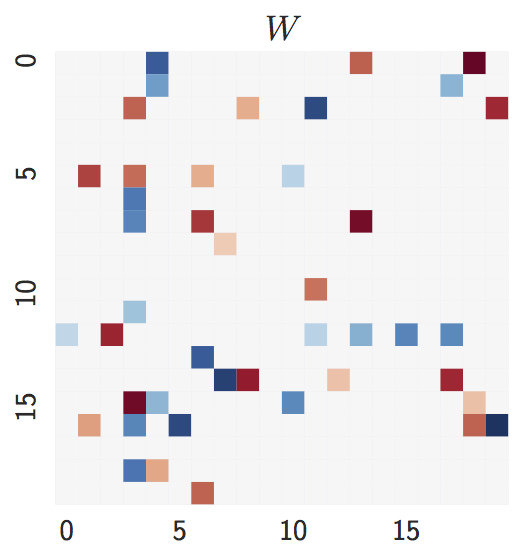

  

• Estimate with n = 1000 samples: lambda = 0, lambda = 0.1, and FGS (baseline).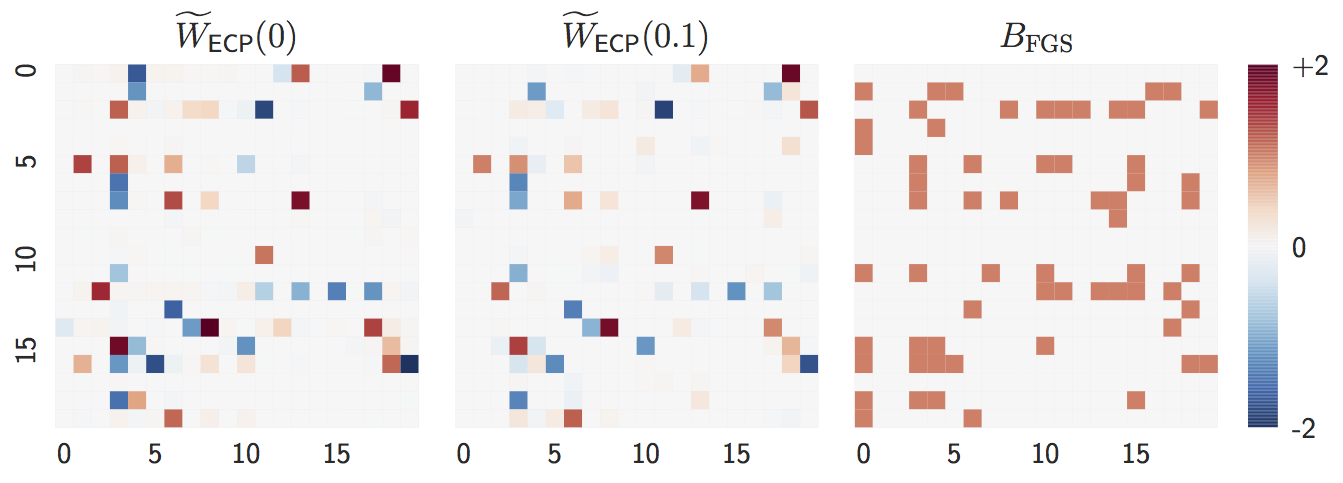

  

  Both lambda = 0 and lambda = 0.1 are close to the ground truth graph when n is large.

• Estimate with n = 20 samples: lambda = 0, lambda = 0.1, and FGS (baseline).

  

  When n is small, lambda = 0 perform worse while lambda = 0.1 remains accurate, showing the advantage of L1-regularization.

Examples: Scale-free graph

• Ground truth: d = 20 nodes, 4d = 80 expected edges.

  

  The degree distribution is significantly different from the Erdos-Renyi graph. One nice property of our method is that it is agnostic about the graph structure.

• Estimate with n = 1000 samples: lambda = 0, lambda = 0.1, and FGS (baseline).

  

  The observation is similar to Erdos-Renyi graph: both lambda = 0 and lambda = 0.1 accurately estimates the ground truth when n is large.

• Estimate with n = 20 samples: lambda = 0, lambda = 0.1, and FGS (baseline).

  

  Similarly, lambda = 0 suffers from small n while lambda = 0.1 remains accurate, showing the advantage of L1-regularization.

Other implementations

• Python: https://github.com/jmoss20/notears
• Tensorflow with Python: https://github.com/ignavier/notears-tensorflow