Synapse.cpp 🧠

A Multi-Layer Perceptron from scratch in pure C++ — no libraries, no magic, just math and memory management.

---

What Is This?

Synapse.cpp is a hand-rolled implementation of a Multi-Layer Perceptron (MLP) written in raw C++17. Every single operation — matrix multiplication, backpropagation, the Adam optimizer — is implemented from first principles. The only things used are <cmath> for exp, log, sqrt, and raw heap-allocated arrays for storage.

This is an educational reference implementation designed to be read and understood, not just used.

---

Architecture Overview

---

How a Neural Network Actually Works — From the Ground Up

Step 1 — The Neuron

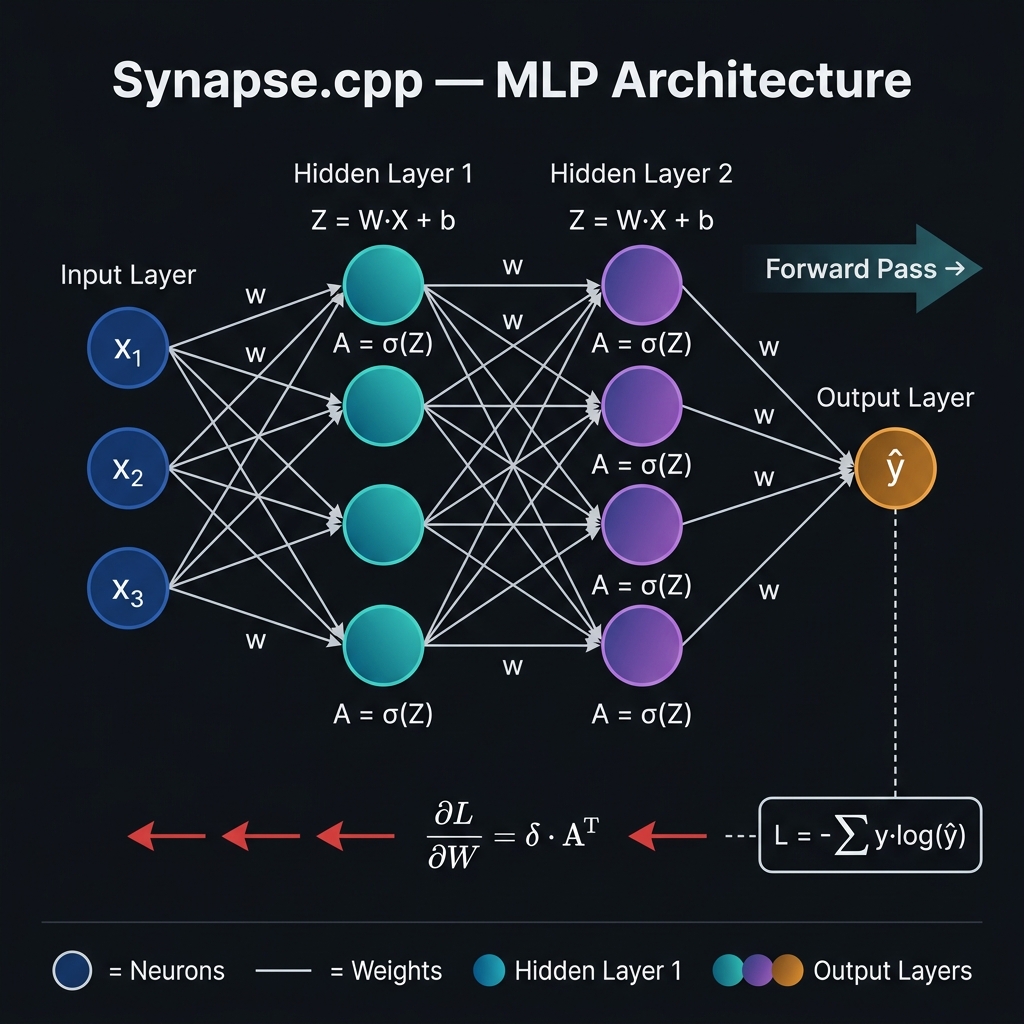
A single neuron receives inputs, multiplies each by a weight, sums them up, adds a bias, and passes the result through an activation function:

z = w₁x₁ + w₂x₂ + ... + wₙxₙ + b    (linear combination)
a = σ(z)                               (activation)

In matrix form for a whole layer processing a whole batch:

Z = X · W + b     (batch_size × units)
A = σ(Z)

Step 2 — The Network (Forward Pass)

An MLP chains multiple layers. Each layer's output A becomes the next layer's input X:

Layer 1:  Z¹ = X  · W¹ + b¹  →  A¹ = σ(Z¹)
Layer 2:  Z² = A¹ · W² + b²  →  A² = σ(Z²)
   ...
Output:   Ẑ  = Aᴸ⁻¹ · Wᴸ + bᴸ →  Ŷ = σ(Ẑ)

Step 3 — The Loss Function

We measure how wrong the predictions are:

Loss	Formula	Used For
MSE	L = (1/2n) Σ (ŷ - y)²	Regression
Binary Cross-Entropy	L = -(1/n) Σ [y·log(p) + (1-y)·log(1-p)]	Binary classification
Categorical Cross-Entropy	L = -(1/n) Σ Σ yᵢⱼ·log(p̂ᵢⱼ)	Multi-class classification

Step 4 — Backpropagation (The Heart of Learning)

This is where the magic happens. We compute how much each weight contributed to the error using the chain rule of calculus — propagating gradients backward through the network.

Output layer gradient:

∂L/∂Z^L = Ŷ - Y          (combined loss + activation gradient for BCE/CCE)

Hidden layer gradient (chain rule):

∂L/∂A^l   = ∂L/∂Z^(l+1) · (W^(l+1))ᵀ
∂L/∂Z^l   = ∂L/∂A^l  ⊙  σ'(Z^l)      (⊙ = element-wise)
∂L/∂W^l   = (A^(l-1))ᵀ · ∂L/∂Z^l
∂L/∂b^l   = Σ ∂L/∂Z^l   (sum over batch)

Step 5 — Weight Update (Optimizer)

SGD with Momentum:

velocity = β·velocity - α·∇W
W        = W + velocity

Adam (Adaptive Moment Estimation):

m = β₁·m + (1-β₁)·∇W        (1st moment — mean)
v = β₂·v + (1-β₂)·∇W²       (2nd moment — variance)
m̂ = m/(1-β₁ᵗ)               (bias correction)
v̂ = v/(1-β₂ᵗ)
W = W - α · m̂/(√v̂ + ε)

---

Full Data Flow — End to End

flowchart TD
    A["🔢 Raw Input Data\n(batch_size × input_features)"]
    B["📊 Mini-Batch Sampler\nShuffle + slice indices"]
    C["⚡ Layer 1: Linear Transform\nZ¹ = X·W¹ + b¹"]
    D["🔀 Layer 1: Activation\nA¹ = ReLU(Z¹)"]
    E["🎲 Dropout Mask\nA¹ *= mask / keep_prob"]
    F["⚡ Layer 2: Linear Transform\nZ² = A¹·W² + b²"]
    G["🔀 Layer 2: Activation\nA² = ReLU(Z²)"]
    H["⚡ Output Layer\nẐ = A²·Wᴸ + bᴸ"]
    I["📤 Output Activation\nŶ = Sigmoid / Softmax / Linear"]
    J["📉 Loss Function\nL = BCE / MSE / CCE"]
    K["🔴 Backward Pass\n∂L/∂Ẑ = Ŷ - Y"]
    L["🔴 Propagate to Layer 2\n∂L/∂Z² = δ·W^T ⊙ σ'(Z²)"]
    M["📐 Compute Gradients\n∂L/∂W = Aᵀ·δ\n∂L/∂b = Σδ"]
    N["⚙️ Adam / SGD Update\nW -= α · m̂/√v̂"]
    O["✅ Convergence Check\nLoss below threshold?"]

    A --> B --> C --> D --> E --> F --> G --> H --> I --> J
    J --> K --> L --> M --> N --> O
    O -->|No — next epoch| B
    O -->|Yes| P["🎉 Trained Model\nReady for inference"]

    style A fill:#1e3a5f,color:#fff
    style J fill:#5f1e1e,color:#fff
    style K fill:#5f1e1e,color:#fff
    style L fill:#5f1e1e,color:#fff
    style M fill:#5f1e1e,color:#fff
    style P fill:#1e5f2a,color:#fff
    style N fill:#4a1e5f,color:#fff

Loading

---

Activation Functions

graph LR
    subgraph Activations["Activation Functions"]
        R["🟦 ReLU\nmax(0, z)\nHidden layers"]
        LR["🟪 Leaky ReLU\nmax(0.01z, z)\nAvoids dying ReLU"]
        S["🟨 Sigmoid\n1/(1+e⁻ᶻ)\nBinary output"]
        T["🟩 Tanh\n(eᶻ-e⁻ᶻ)/(eᶻ+e⁻ᶻ)\nRegression hidden"]
        SM["🟥 Softmax\neᶻⁱ/Σeᶻʲ\nMulti-class output"]
        LN["⬜ Linear\nz\nRegression output"]
    end

Loading

---

Weight Initialization Strategies

Method	Formula	Best For
Xavier Uniform	U[-√(6/(fᵢₙ+fₒᵤₜ)), +√(6/(fᵢₙ+fₒᵤₜ))]	Sigmoid / Tanh
He Normal	N(0, √(2/fᵢₙ))	ReLU layers
Random Uniform	U[-0.5, 0.5]	Quick experiments
Random Normal	N(0, 0.01)	Small-scale nets

---

Project Structure

Synapse.cpp/
├── Matrix.hpp      ← Matrix class declaration (all operations)
├── Matrix.cpp      ← Matrix implementation (dot, broadcast, init...)
├── MLP.hpp         ← MLP class: layers, configs, enums
├── MLP.cpp         ← Full forward pass, backprop, Adam, SGD, training loop
├── main.cpp        ← 4 live demos: XOR, Circle, Sine, Blobs
└── README.md       ← You are here

---

Building and Running

Requirements: Any C++17-compatible compiler (GCC, Clang, MSVC).

# Compile
g++ -O2 -std=c++17 main.cpp Matrix.cpp MLP.cpp -o synapse

# Run all 4 demos
./synapse

# Windows
g++ -O2 -std=c++17 main.cpp Matrix.cpp MLP.cpp -o synapse.exe
.\synapse.exe

---

Demo Experiments

Demo 1 — XOR Problem

The XOR function is not linearly separable (no single line can divide the classes). A two-layer MLP solves it perfectly.

Input	Expected	Predicted
(0, 0)	0	≈ 0.01
(0, 1)	1	≈ 0.99
(1, 0)	1	≈ 0.99
(1, 1)	0	≈ 0.02

• Architecture: 2 → 8 → 1
• Loss: Binary Cross-Entropy
• Optimizer: Adam

Demo 2 — Circle Dataset

Points inside radius 0.6 → class 1. Non-linear boundary requires multiple layers.

• Architecture: 2 → 16 → 8 → 1
• Expected accuracy: ~98%

Demo 3 — Sine Regression

Approximate f(x) = sin(2πx) + noise from 300 noisy samples.

• Architecture: 1 → 64 → 64 → 1 (Tanh hidden, Linear output)
• Expected MSE: < 5×10⁻⁴

Demo 4 — 3-Class Gaussian Blobs

Three overlapping Gaussian clusters. Tests Softmax + Categorical Cross-Entropy.

• Architecture: 2 → 32 → 16 → 3
• Expected accuracy: ~99%

---

Feature Matrix

Feature	Status
Arbitrary depth & width	✅
ReLU, Leaky-ReLU, Sigmoid, Tanh, Softmax	✅
Linear activation (regression)	✅
MSE loss	✅
Binary Cross-Entropy loss	✅
Categorical Cross-Entropy loss	✅
SGD with momentum	✅
Adam optimizer	✅
Xavier weight init	✅
He weight init	✅
Dropout regularisation	✅
Gradient clipping	✅
Mini-batch training	✅
Numerically stable softmax	✅
Bias-corrected Adam	✅
Training / eval mode	✅
Accuracy metric	✅
Loss history tracking	✅
Model summary printer	✅
Zero external dependencies	✅

---

Matrix Engine

The Matrix class at the heart of Synapse.cpp implements:

• Storage: flat double* array (row-major), allocated with new[]
• Ownership: RAII — destructor calls delete[], copy constructor deep-copies
• Move semantics: Matrix(Matrix&&) transfers ownership without copying
• Operations: +, -, * (element-wise), dot() (matmul), transpose(), broadcastAdd(), sum(axis), mean(axis), exp(), log(), clip(), argmax()
• Init: Xavier uniform, He normal, random uniform, random normal (Box-Muller)

---

Math Reference

Backpropagation Derivation (MSE Loss)

L = (1/2n) ||Ŷ - Y||²

∂L/∂Ŷ  = (Ŷ - Y)/n                    ← output gradient

For layer l (going backwards):
∂L/∂Zˡ = ∂L/∂Aˡ ⊙ σ'(Zˡ)            ← activation gradient
∂L/∂Wˡ = (Aˡ⁻¹)ᵀ · ∂L/∂Zˡ           ← weight gradient
∂L/∂bˡ = Σᵢ ∂L/∂Zˡᵢ                  ← bias gradient (sum over batch)
∂L/∂Aˡ⁻¹ = ∂L/∂Zˡ · (Wˡ)ᵀ           ← propagate to previous layer

Adam Update Rule

t ← t + 1
mᵥᵥ ← β₁·mᵥᵥ + (1-β₁)·∇W
vᵥᵥ ← β₂·vᵥᵥ + (1-β₂)·∇W²
m̂   ← mᵥᵥ / (1 - β₁ᵗ)
v̂   ← vᵥᵥ / (1 - β₂ᵗ)
W   ← W - α · m̂ / (√v̂ + ε)

Defaults: β₁=0.9, β₂=0.999, ε=1e-8

---

License

MIT — see LICENSE.

---

Built entirely from scratch. No PyTorch. No TensorFlow. No Eigen. Just C++.