

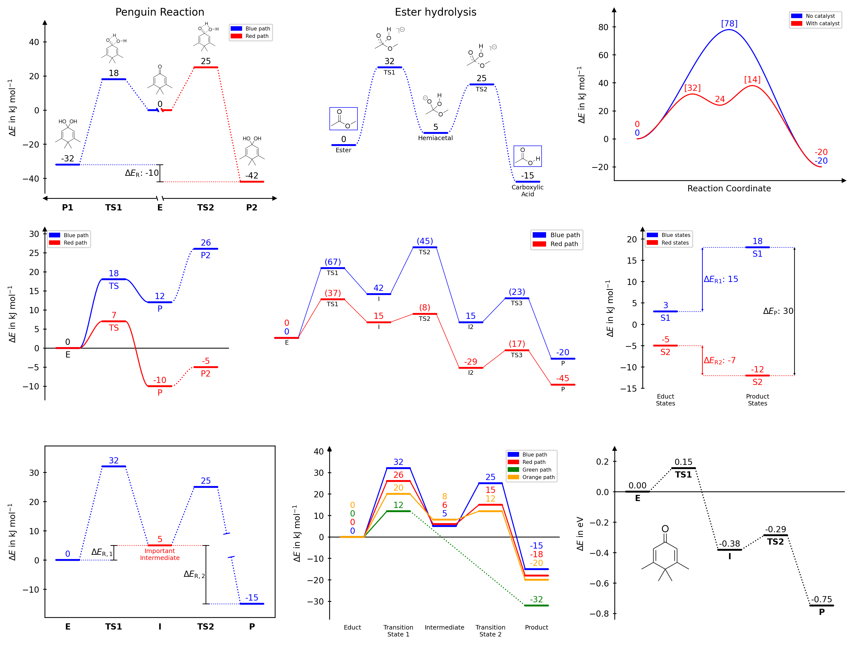
A Python package for creating publication-quality reaction energy diagrams with Matplotlib.
You can use the latest release by installing it from PyPi:
pip install chemdiagramsRequirements: Python ≥ 3.10, Matplotlib ≥ 3.7, NumPy ≥ 1.23, SciPy ≥ 1.10
- Multiple reaction paths on a single diagram
- Nine connector styles: dotted, solid, broken dotted, broken solid, spline dotted, spline solid, broken spline dotted, broken spline solid or none
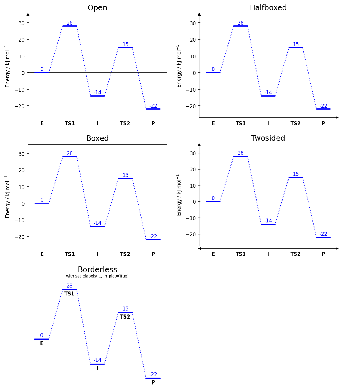
- Five diagram styles:
open,halfboxed,boxed,twosided,borderless - Automatic, stacked, naïve, and averaged energy label placement (numbering)
- Custom text labels for each path at each position
- Energy difference bars with optional whiskers
- Axis break markers for both x and y axes
- Image placement along the diagram, with automatic collision avoidance
- Full access to the underlying Matplotlib objects for fine-grained customisation
- Customizable templates for consistent styling across multiple diagrams
Full documentation with usage instructions, examples, and API reference is available at https://tonner-zech-group.github.io/chem-diagrams/.
| Method | Description |
|---|---|
draw_path() |
Add a reaction pathway to the diagram |
add_path_labels() |
Add text labels for a specific path at the respective x-positions |
merge_plateaus() |
Visually merge two coincident energy levels at a shared x-position |
draw_difference_bar() |
Draw a vertical energy difference arrow between two levels |
set_xlabels() |
Set text labels for the reaction states along the x-axis |
set_diagram_style() |
Change the overall visual style (open, boxed, halfboxed, twosided, borderless) |
add_numbers_naive() |
Annotate each energy level directly above its bar |
add_numbers_stacked() |
Stack labels above the highest state to avoid overlap |
add_numbers_auto() |
Automatically distribute labels to minimise clutter (recommended) |
add_numbers_average() |
Annotate with the mean energy across all paths at each x-position |
modify_number_values() |
Modify existing energy annotations by adding or subtracting values |
add_xaxis_break() |
Add a break marker on the x-axis |
add_yaxis_break() |
Add a break marker on the y-axis |
add_image_in_plot() |
Place a single image at an explicit data-coordinate position |
add_image_series_in_plot() |
Place a series of images along the diagram with automatic collision avoidance |
legend() |
Add a legend for all named paths |
show() |
Display the figure |
General settings like figure size, margins and font size are usually handled automatically by EnergyDiagram, but can be customised at construction.
dia = EnergyDiagram(
    extra_x_margin=(0, 0.5),   # additional margin in x (data units)
    extra_y_margin=(0, 0.2),   # additional margin in y (relative units)
    figsize=(6, 4),            # explicit figure size in inches
    width_limit=7,             # maximum width in inches if figure is scaled automatically (figsize is not set, default: None)
    fontsize=10,               # default font size for all text elements (can be overridden individually)
    style="halfboxed",         # diagram style (see later sections for details)
    dpi=150,                   # resolution in dots per inch for raster formats (ignored for vector formats like PDF, svg and eps)
)Figures can be saved in any format supported by Matplotlib. The bbox_inches="tight" option is recommended to adjust whitespace around the figure.
dia.fig.savefig("diagram.png", dpi=300, bbox_inches="tight")
dia.fig.savefig("diagram.pdf", bbox_inches="tight")Each call to draw_path adds one reaction pathway. Paths can span different x-ranges, allowing branching or incomplete pathways.
dia = EnergyDiagram()

dia.draw_path(
    x_data=[0, 1, 2, 3, 4, 5],
    y_data=[0, -13, 22, 75, 39, 20],
    color="blue",
    path_name="Pathway A",      # name appears in the legend
    linetypes=[2, 3, 4, -1, 0], # connector style per segment
)

dia.draw_path(
    x_data=[0, 1, 2, 3, 5],
    y_data=[0, -25, 20, 50, 6],
    color="red",
    path_name="Pathway B",
)

dia.legend(fontsize=7)
dia.add_numbers_auto()
dia.set_xlabels(["A", "B", "C", "D", "E", "F"])
dia.ax.set_ylabel("Energy / kJ mol$^{-1}$", fontsize=8)

dia.fig.savefig(os.path.join("..","docs","img","example_multipaths.png"),format="png", bbox_inches="tight")
dia.show()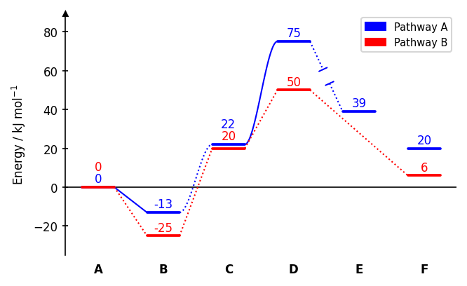
Connector styles (linetypes):
| Value | Style |
|---|---|
0 |
no connector |
1 |
dotted line (default) |
-1 |
dotted line with gap |
2 |
solid line |
-2 |
solid line with gap |
3 |
dotted cubic spline |
-3 |
dotted cubic spline with gap |
4 |
solid cubic spline |
-4 |
solid cubic spline with gap |
A single integer applies the same style to all segments. A list applies styles individually.
The width of a plateau can be adjusted with the keyword width_plateau. It can be a float in data units (Default is 0.5). Furthermore, the linewidth of the plateaus can be set via lw_plateau to one of the strings "plateau" or "connector" to refer to predefined values or a number. Also the linewidth of the connectors can be set via lw_connector. The gap of broken line styles can be adjusted with gap_scale, which is a scaling factor for the gap size (default is 1). It can be a single number applied to all segments, or a sequence with one value per segment. Example:
dia = EnergyDiagram()

dia.draw_path(
    x_data=[0, 1, 2, 3, 4, 5],
    y_data=[0, -13, 22, 75, 39, 20],
    color="blue",
    path_name="Pathway A",
    width_plateau=0.3,
    lw_plateau="connector",
    lw_connector=0.4,
)

dia.draw_path(
    x_data=[0, 1, 2, 3.5, 5],
    y_data=[0, -25, 5, 30, 6],
    color="red",
    path_name="Pathway B",
    linetypes=[4, 4, -4, -3],
    width_plateau=0,
    lw_connector=0.7,
    gap_scale=[0,0, 0.5, 1.5],
)

dia.add_numbers_auto()
dia.legend(fontsize=7)
dia.set_xlabels(["A", "B", "C", "D", "E", "F"])
dia.ax.set_ylabel("Energy / kJ mol$^{-1}$", fontsize=8)

dia.show()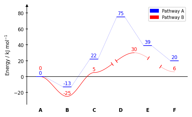
Text labels can be added for each path at each position with add_path_labels. This is useful to label specific states along a pathway.
dia.add_path_labels(
    "Pathway A",                        # Name of the path, for which the labels are to be added
    ["A", "B", "C", "D", None, "F"],    # Labels for the path, None can be used to not display a label at a specific position
    fontsize=6,                         # Font size for the labels (uses diagram default if None)
    color="black",                      # Color for the labels (uses diagram default if None)
    weight="bold"                       # Font weight for the labels (uses "normal" if None)
)
Example:
dia = EnergyDiagram()

dia.draw_path(
    x_data=[0, 1, 2, 3, 4, 5],
    y_data=[0, -13, 25, 75, 39, 20],
    color="blue",
    path_name="Pathway A",
    linetypes=3,                # connector style for all segments as an int
)

dia.draw_path(
    x_data=[0, 1, 2, 3, 5],
    y_data=[0, -25, 15, 50, -8],
    color="red",
    path_name="Pathway B",
    linetypes=3
)

dia.add_path_labels(
    "Pathway A",
    [None, "I1", "I2", "I3", "I4", "P"], # None for no label
    fontsize=7,
)

dia.add_path_labels(
    "Pathway B",
    ["E", "I1", "I2", "I3", "P"],
    weight="bold"
)
dia.lines["Pathway B"].labels["0.0"].set_color("black") # Set the color of the first label of Pathway B to black

dia.legend(fontsize=7)
dia.add_numbers_auto()
dia.ax.set_ylabel("Energy / kJ mol$^{-1}$", fontsize=8)

dia.fig.savefig(os.path.join("..","docs","img","example_path_labels.png"),format="png", bbox_inches="tight")
dia.show()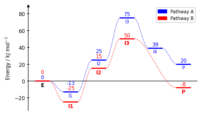
dia.set_diagram_style("halfboxed") # open | halfboxed | boxed | twosided | borderlessThe style can be set at construction via EnergyDiagram(style="boxed") or changed afterwards with set_diagram_style.
By default labels are placed below the x-axis:
dia.set_xlabels(["A", "TS", "B"], fontsize=8, weight="normal")Pass in_plot=True to render them inside the plot area, directly below the lowest energy state.
dia.set_xlabels(["A", "TS", "B"], in_plot=True)Use labelplaces to set explicit x-coordinates instead of the default sequential placement:
dia.set_xlabels(["A", "TS", "B"], labelplaces=[0, 2, 3])Four numbering strategies are available. Call them after all paths have been drawn.
dia.add_numbers_auto()                   # distributes labels to avoid overlaps (recommended)
dia.add_numbers_stacked()                # stacks all labels above the highest state
dia.add_numbers_naive()                  # places each label directly above its bar
dia.add_numbers_average()                # displays the mean energy across all paths
To restrict the numbering to a specific range of x-values, pass x_min_max=(x_min, x_max) to the numbering method.
dia.add_numbers_auto(x_min_max=(1, 4))To exclude numbers for a specific path, pass show_numbers=False to draw_path for that path.
dia.draw_path(..., show_numbers=False)It is possible to adjust the fontsize of the numbers via the fontsize parameter of the numbering methods, or by direct Matplotlib access after drawing (see below).
dia.add_numbers_auto(..., fontsize=6)All numbers are automatically rounded to integers by default. The number of decimal places can be manually set with the n_decimals parameter of the numbering methods.
dia.add_numbers_auto(..., n_decimals=2)For add_numbers_average, the color of the labels can be set with the color parameter.
dia.add_numbers_average(color="red")Example:
dia = EnergyDiagram(style="borderless", figsize=(3,2))

dia.draw_path(
    x_data=[0, 1, 2, 3],
    y_data=[1, 1, 1, 1],
    color="red",
)
dia.draw_path(
    x_data=[0, 1, 2, 3],
    y_data=[-25, -25, -25, -25],
    color="blue",
)
dia.draw_path(
    x_data=[0, 1, 2, 3],
    y_data=[15, 15, 15, 15],
    color="green",
)
dia.draw_path(
    x_data=[0, 1, 2, 3],
    y_data=[3, 3, 3, 3],
    color="orange",
)

dia.add_numbers_auto(x_min_max=0)
dia.add_numbers_stacked(x_min_max=1)
dia.add_numbers_naive(x_min_max=2)
dia.add_numbers_average(x_min_max=3, color="black")

dia.set_xlabels([
    "Auto\nNumbering",
    "Stacked\nNumbering",
    "Naive\nNumbering",
    "Average\nNumbering"
],
    fontsize=6,
    weight="normal"
)

dia.fig.savefig(os.path.join("..","docs","img","example_numbering.png"),format="png", bbox_inches="tight")
dia.show()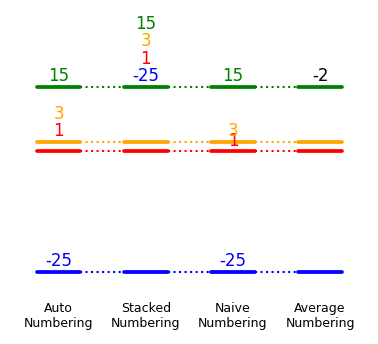
Existing energy annotations can be modified by adding or subtracting values with modify_number_values(). This is useful to annotate energy differences (e.g., activation energies or reaction energies) by subtracting the relevant reference energy from the target energy. The resulting number is caclulated for each path as follows:
base_value + sum(energies at x_add) - sum(energies at x_subtract)
dia.modify_number_values(
    x=2,                        # x-position of the number to modify in data coordinates
    x_add=[2],                  # list of x-positions (or single x-position) to add to the number; None for no addition
    x_subtract=[1],             # list of x-positions (or single x-position) to subtract from the number; None for no subtraction
    base_value=0,               # value to add or subtract directly (e.g., to convert units); default is 0
    brackets=["(", ")"],        # pair of strings to add as brackets around the modified number (e.g., ["[", "]); None for no brackets")
    n_decimals=0,               # number of decimals to round the modified number to (default is 0)
    include_paths=None,         # list of path names to include in the modification; None to include all paths
    exclude_paths=None,         # list of path names to exclude from the modification; None includes all paths
    n_decimals=0,               # number of decimals to round the modified number to (default is 0)
)
Example:
dia = EnergyDiagram()

dia.draw_path(
    x_data=[0, 1, 2, 3, 4],
    y_data=[0, 28, -14, 15.3, -22],
    color="blue",
    path_name="Blue path",
)

dia.draw_path(
    x_data=[0, 1, 2, 3, 4],
    y_data=[0, 25, 6, 15.2, -18],
    color="red",
    path_name="Red path",
)

dia.add_numbers_auto()

dia.modify_number_values(
    x=1,
    x_add=1,
    x_subtract=0,
    include_paths=["Blue path"],
    brackets=("[", "]"),
)

dia.modify_number_values(
    x=3,
    x_add=[3],
    x_subtract=[2],
    n_decimals=1,
)

dia.fig.savefig(os.path.join("..","docs","img","example_number_modification.png"),format="png", bbox_inches="tight")
dia.show()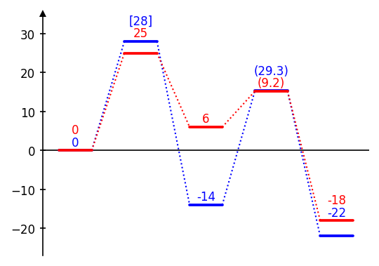
draw_difference_bar draws a vertical bar between two energy levels at a specified x-position, with optional horizontal whiskers to indicate the reference points for the difference.
dia = EnergyDiagram(style="halfboxed")
dia.draw_path(x_data=[0,1,2,3,4,5], y_data=[0,-13,22,75,39,-25], color="blue")

dia.draw_difference_bar(
    x=3,
    y_start_end=(-25, 0),
    description=r"$\Delta E_\mathrm{R}$: ",
    color="black",
    arrowstyle="|-|",               # arrow style (default: "|-|")
    x_whiskers=(5, 0),              # x-positions for whisker endpoints; None to omit
    whiskercolor="blue",            # whisker color (defaults to bar color if omitted)
    left_side=True,                 # place bar and text on the left of x
    add_difference=True,            # automatically append the difference value rounded to an integer to description
    fontsize=8,                     # font size for the label (uses diagram default if None)
    diff=None,                      # horizontal offset of text (auto-computed if None)
)
dia.bars[0].whisker_1.set_color("black") # Set the color of the first whisker of the firstly drawn bar to black

dia.set_xlabels(["A", "B", "C", "D", "E", "F"])
dia.add_numbers_auto()
dia.ax.set_ylabel("Energy / kJ mol$^{-1}$", fontsize=8)

dia.fig.savefig(os.path.join("..","docs","img","example_diffbar.png"),format="png", bbox_inches="tight")
dia.show()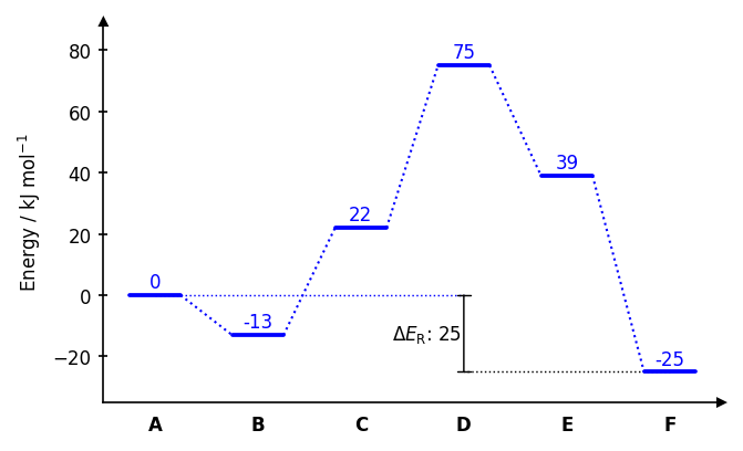
Axis breaks can be added to either axis to indicate a discontinuity in the scale. The break is drawn at the specified x or y position in data coordinates, with a gap in the axis line and diagonal tick marks.
dia = EnergyDiagram(style="twosided")
dia.draw_path(x_data=[0,1,2,3,4,5], y_data=[0,-13,22,75,39,-25], color="blue")

dia.add_yaxis_break(y=5)
dia.add_xaxis_break(
    x=2,                        # x-position of the break in data coordinates
    gap_scale=2,                # scaling factor for the gap in the axis line (default: 1)
    stopper_scale=1.5,          # scaling factor for the size of the stopper tick marks (default: 1)
    angle=60,                   # angle of the stopper tick marks in degrees (default: 60)
)
dia.set_xlabels(["A", "B", "C", "D", "E", "F"])
dia.add_numbers_auto()
dia.ax.set_ylabel("Energy / kJ mol$^{-1}$", fontsize=8)

dia.fig.savefig(os.path.join("..","docs","img","example_breaks.png"),format="png", bbox_inches="tight")
dia.show()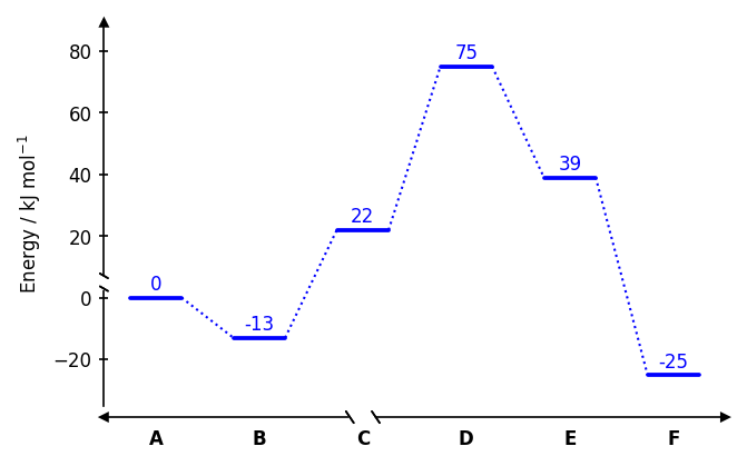
Note: x-axis breaks are not compatible with the "open" and "borderless" styles. y-axis breaks are not compatible with the "borderless" style.
When two paths share the same energy level at the same x-position, merge_plateaus
replaces both full-width bars with two shorter half-bars separated by a gap, with
diagonal tick marks to indicate degeneracy.
dia = EnergyDiagram(style="twosided")
dia.draw_path(x_data=[0, 1, 2], y_data=[10, 55, 0], color="blue", path_name="Path A")
dia.draw_path(x_data=[2, 3, 4], y_data=[0, 50, -5], color="red",  path_name="Path B")

# Both paths share y=0 at x=2
dia.merge_plateaus(
    x=2,                        # x-position of the shared plateau in data coordinates
    path_name_left="Path A",    # name of the left path to merge (must match the path_name used in draw_path)
    path_name_right="Path B",   # name of the right path to merge (must match the path_name used in draw_path)
    gap_scale=1.0,              # width of the gap between the two half-bars
    stopper_scale=1.0,          # size of the diagonal tick marks
    angle=30,                   # angle of the tick marks in degrees
)

dia.add_numbers_auto()
dia.set_xlabels(["P1", "TS1", "E", "TS2", "P2"])
dia.ax.set_ylabel("Energy / kJ mol$^{-1}$", fontsize=8)

dia.fig.savefig(os.path.join("..","docs","img","example_merge_plateaus.png"),format="png", bbox_inches="tight")
dia.show()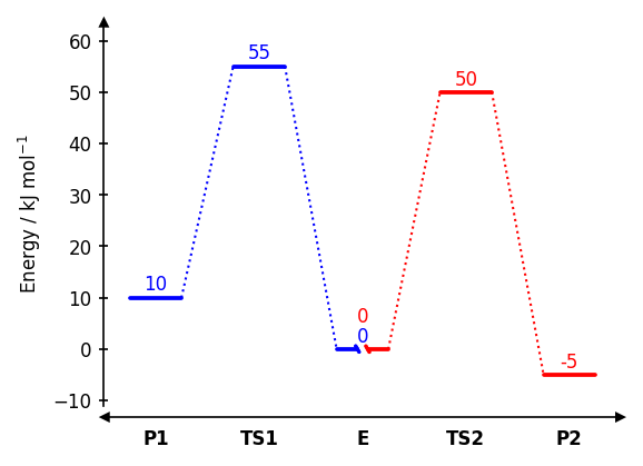
Both paths must already be drawn and must have exactly the same y-value at x.
add_image_in_plot places a single image at an explicit position in data coordinates. SVG and EPS formats are not supported; PNG and JPEG work best.
# Single image at a fixed position
dia.add_image_in_plot(
    "path/to/image.png",
    position=(2, 30),               # (x, y) in data coordinates
    img_name="my_image",            # optional name to access the artist later via dia.images
    width=0.5,                      # width in axis units;
                                    # if omitted, height is used to scale or width is set automatically
    height=None,                    # height in axis units
    horizontal_alignment="center",  # "center", "left", or "right" relative to position
    vertical_alignment="center",    # "center", "top", or "bottom" relative to position
    framed=True,                    # draw a border rectangle around the image
    frame_color="black",            # color of the border
)
Example:
import os.path

dia = EnergyDiagram(style="open")

penguin = os.path.join("figures", "penguin.png")

dia.draw_path(
    [0, 1, 2, 3, 4], [0, 0.154, -0.382, -0.287, -0.748], "black",
)

dia.add_numbers_auto(
    n_decimals=2
)

dia.ax.set_ylabel(r"$\Delta E$ in eV", fontsize=8)
dia.set_xlabels(["E", "TS1", "I", "TS2", "P"], in_plot=True)

dia.add_image_in_plot(
    penguin,
    position=(0.6, -0.4),
    height=0.4
)

dia.fig.savefig(os.path.join("..", "docs", "img", "title", "image_8.png"), dpi=300, bbox_inches="tight")
dia.fig.savefig(os.path.join("..","docs","img","example_single_image.png"),format="png", bbox_inches="tight")
dia.show()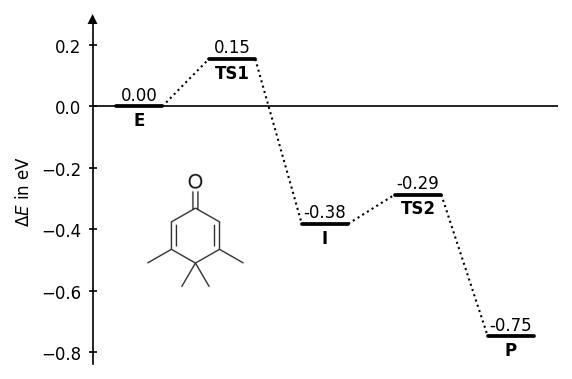
add_image_series_in_plot places one image per reaction state, with automatic collision avoidance against energy numbers and x-axis labels. SVG and EPS formats are not supported; PNG and JPEG work best.
# Series of images distributed automatically along the diagram
dia.add_image_series_in_plot(
    ["img0.png", "img1.png", "img2.png", "img3.png", "img4.png"],
    img_x_places=[0, 1, 2, 3, 4],        # which x positions to place images at;
                                         # defaults to 0,1,2,... if omitted
    y_placement="auto",                  # "auto", "top", or "bottom" — can also be a list
                                         # per image, e.g. ["auto", "top", "auto", "bottom", "auto"]
                                         # "auto" automatically decides whether it is placed on top or bottom
    y_offsets=5,                         # additional vertical offset in data units, scalar or per-image list
    img_series_name="my_series",         # optional name to access artists later via dia.images
    width=0.6,                           # scalar applies to all; pass a list for per-image widths
                                         # if omitted, height is used to scale or width is set automatically
    height=None,                         # scalar applies to all; pass a list for per-image heights
    framed=False,                        # scalar or per-image list of bools
    frame_colors="black",                # scalar or per-image list of color strings
)
Example:
import os.path

ester_1 = os.path.join("figures", "ester_1.png")
ester_2 = os.path.join("figures", "ester_2.png")
ester_3 = os.path.join("figures", "ester_3.png")
ester_4 = os.path.join("figures", "ester_4.png")
ester_5 = os.path.join("figures", "ester_5.png")

dia = EnergyDiagram(
    style="borderless",
    extra_y_margin=(0, 0.25),
)

dia.draw_path(
    [0,1,2,3,4], [0, 32, 5, 25, -15], "blue",
    path_name="Blue path",
    linetypes=3
)

dia.add_numbers_average(color="black")
dia.set_xlabels(["Ester", "TS1", "Hemiacetal", "TS2", "Carboxylic\nAcid"], in_plot=True, fontsize=6, weight="normal")

dia.add_image_series_in_plot(
    [ester_1, ester_2, ester_3, ester_4, ester_5],
    y_placement="top",
    width=[0.6, 0.7, 0.6, 0.7, 0.6],
    y_offsets=1.5,
    framed=[True, False, False, False, True],
    frame_colors="blue"
)

dia.ax.set_title("Ester hydrolysis", fontsize=10)
dia.show()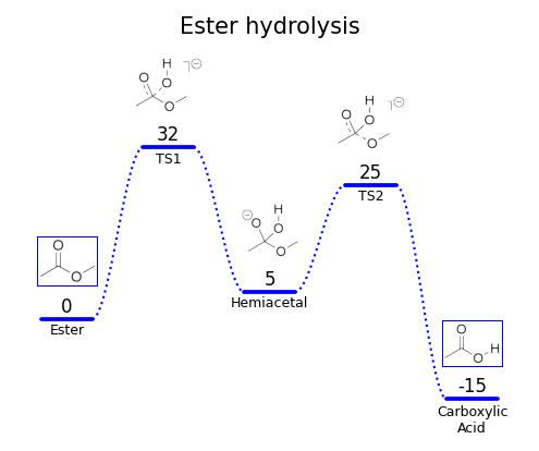
All Matplotlib artists are accessible after drawing for direct customisation. Most importantly, the figure and axes objects are available as dia.fig and dia.ax for direct Matplotlib calls. This allows to set axis labels, titles, limits, or any other Matplotlib property before saving or showing the figure.
dia.draw_path(..., path_name="My Path")
dia.add_numbers_auto()
figure = dia.fig  # Matplotlib Figure object
axes = dia.ax     # Matplotlib Axes object
dia.ax.set_ylabel("Energy / kJ mol$^{-1}$", fontsize=10)
dia.fig.savefig("diagram.png", dpi=300, bbox_inches="tight")
dia.ax.set_title("My Energy Diagram", fontsize=12)All objects of a path (plateaus and connectors) are stored in dia.lines and can be accessed by the path name and x-position. If a path was drawn with width_plateau=0, it has no plateau objects.
# Plateau and connector lines
# Keys are x-position strings formatted to one decimal place
plateau   = dia.lines["My Path"].plateaus["2.0"]     # Plateau of "My Path" at x=2
connector = dia.lines["My Path"].connections["1.5"]  # Connector of "My Path" between x=1 and x=2 (x=1.5)
plateau.set_color("green")
connector.set_linestyle("--")
Via dia.lines it is also possible to access the path labels added with add_path_labels by their x-position.
path_labels = dia.lines["My Path"].labels["2.0"]       # Label of "My Path" at x=2
path_labels.set_color("blue")All energy labels are stored in dia.numbers and can be accessed by path name and x-position.
# Energy labels
label = dia.numbers["My Path"]["2.0"]                # Number of "My Path" at x=2
label.set_color("red")
label.set_fontsize(12)Components of difference bars are stored in dia.bars and can be accessed by the order of bar placement (e.g., dia.bars[0] for the first one, dia.bars[1] for the second one...). A difference bar consists of the vertical bar (bar), an optional text label (text), and optional horizontal whiskers (whisker_1, whisker_2).
first_bar = dia.bars[0]                                 # First difference bar added to the diagram
first_bar.text.set_color("red")                         # Set the color of the text label of the first bar to red
first_bar.bar.arrow_patch.set_color("green")            # Set the color of the vertical bar of the first bar to green
first_bar.whisker_2.set_color("blue") # Set the color of the second whisker of the first bar to blueStyle objects for axes, arrows, and x-labels are stored in dia.ax_objects and can be accessed by their type and x-position (for x-labels). x-labels (x_labels) are only stored if they were created with set_xlabels(..., in_plot=True).
# Set color for x label at x=2.0
dia.ax_objects.x_labels["2.0"].set_color("purple")
Arrows (arrows) are stored by their name, which is "x_arrow" ("x_arrow_left" and "x_arrow_right" in case of style="twosided") or "y_arrow" for the axis arrows.
# Axis arrows (twosided/open/halfopen styles)
dia.ax_objects.arrows["x_arrow"].set_color("gray")
Axis break components are stored in xaxis_breaks and yaxis_breaks by their x or y position as a string formatted to one decimal place. Each break consists of two stopper lines (stopper_1, stopper_2) and a whitespace rectangle (whitespace) that covers the gap in the axis line. In case of "style=boxed" there are two break objects accessible via a dictionary keyed by "left" and "right" or "bottom" and "top".
# Axis break artists if style is not "boxed"
dia.ax_objects.xaxis_breaks["2.0"].stopper_1.set_color("red")
dia.ax_objects.yaxis_breaks["5.0"].whitespace.set_facecolor("lightyellow")

# Axis break artists if style is "boxed"
dia.ax_objects.xaxis_breaks["2.0"]["top"].stopper_1.set_color("red")
dia.ax_objects.yaxis_breaks["5.0"]["left"].stopper_1.set_color("blue")
The horizontal line when using diagram style "open" is stored as x_axis.
# Hide the horizontal line in hopen style
dia.ax_objects.axes["x_axis"].set_visible(False)Images are stored in dia.images by their name, which is either the img_name passed to add_image_in_plot or the img_series_name passed to add_image_series_in_plot. The former is stored as an ImageObject, which has an image attribute for the Matplotlib AxesImage and a borders dictionary for the frame lines keyed by "top", "bottom", "left", and "right". The latter is stored as a dictionary keyed by x-position as a string formatted to one decimal place, with each entry being an ImageObject.
# Access a single image artist added with add_image_in_plot
img_object = dia.images["my_image"]                  # ImageObject
img_object.image.set_alpha(0.8)                      # AxesImage — any matplotlib imshow property
img_object.borders["top"].set_color("red")           # frame border lines, keyed by "top",
img_object.borders["left"].set_linewidth(2)          # "bottom", "top", "left", "right"

# Access images added with add_image_series_in_plot
series = dia.images["my_series"]                     # dict keyed by x-position as "x.x" string
img_at_x1 = series["1.0"]                            # ImageObject at x=1
img_at_x1.image.set_alpha(0.5)
img_at_x1.borders["bottom"].set_linestyle("--")
Examples can be found in the (documentation). A set of even more examples is available in examples/example_use.ipynb. The latter, however, is not actively maintained anymore and may be outdated with respect to the latest version of the package.
Templates allow you to customize default settings and diagram behavior for consistent styling across multiple diagrams. They provide a way to override constants, add startup modifications, and define custom methods for diagram creation.
chemdiagrams provides pre-configured templates. The default template automatically used if not specified otherwise is BaseTemplate. To use a template, pass it as a parameter when creating an EnergyDiagram:
from chemdiagrams import EnergyDiagram
from chemdiagrams.templates.example_template import ExampleTemplate

# Create a diagram with ExampleTemplate
dia = EnergyDiagram(template=ExampleTemplate())
dia.draw_path([0, 1, 2], [0, 10, -5], color="blue")
Available templates:
BaseTemplate— The default template with no modificationsTonnerZechTemplate— Template style for Tonner & Zech group diagramsExampleTemplate— Example template for demonstration purposes
__init__() — Override to customize default constants (link to constants).
startup(diagram) — Called at the beginning of diagram creation. Use to modify the diagram object before any plotting occurs. Must return the modified diagram.
Custom static methods — Define any custom post-processing methods you need for diagram modifications.
To create your own template, subclass BaseTemplate and override the __init__ and/or startup methods. Furthermore, static methods can be defined for automating common tasks. How this can be realized is shown with an example template.
from chemdiagrams.templates.base_template import BaseTemplate

class ExampleTemplate(BaseTemplate):
    def __init__(self):
        """
        Modyfy constants for Example style diagrams here.
        e.g. self.constants.DISTANCE_TEXT_DIFFBAR = 0.05
        """
        super().__init__()
        # Change constants here
        self.constants.WIDTH_PLATEAU = 0.4
        self.constants.LW_CONNECTOR = 0.6

    def startup(self, diagram):
        """
        Startup function to be called at the beginning of the plotting process
        Here you can modify the diagram object before any plotting is done.
        """
        diagram = super().startup(diagram)
        # Change diagram here
        diagram.set_diagram_style("open")
        diagram.ax_objects.axes["x_axis"].remove()
        diagram.ax.grid(True, which="both", axis="y", ls="--", lw=0.5, zorder=-1)
        return diagram

    # Example of a custom function to modify the diagram after plotting
    @staticmethod
    def color_all_numbers(diagram, color):
        """Set the colors of all numbers to the specified color"""
        for path_numbers in diagram.numbers.values():
            for number in path_numbers.values():
                number.set_color(color)
        return diagram
Then place your custom template in the src/chemdiagrams/templates directory for reuse across projects. It can be imported with from chemdiagrams.templates.my_custom_template import MyCustomTemplate. You can use the custom template by passing it to EnergyDiagram:
from chemdiagrams import EnergyDiagram
from chemdiagrams.templates.my_custom_template import MyCustomTemplate

dia = EnergyDiagram(template=MyCustomTemplate())
...
You can also create the template directly in your script or notebook without saving it as a separate file, and pass an instance of the class to EnergyDiagram in the same way.
Example of using the custom static method defined in the template:
from chemdiagrams import EnergyDiagram
from chemdiagrams.templates.example_template import ExampleTemplate
import os.path

dia = EnergyDiagram(template=ExampleTemplate())

dia.draw_path(
    x_data=[0, 1, 2, 3, 4],
    y_data=[0, 28, -14, 15.3, -22],
    color="blue",
    path_name="Blue path",
)
dia.draw_path(
    x_data=[0, 1, 2, 3, 4],
    y_data=[0, 25, 6, 15.2, -18],
    color="red",
    path_name="Red path",

)
dia.add_numbers_auto()
dia.set_xlabels(["E", "TS1", "I", "TS2", "P"])
dia.ax.set_ylabel("Energy / kJ mol$^{-1}$", fontsize=8)

dia = ExampleTemplate.color_all_numbers(dia, color="purple")

dia.fig.savefig(os.path.join("..","docs","img","example_template.png"),format="png", bbox_inches="tight")
dia.show()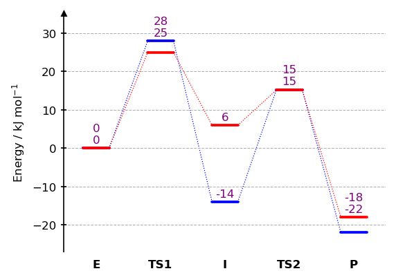
If you use chemdiagrams in published work, please consider citing the repository:
Tim Bastian Enders, chemdiagrams, https://github.com/Tonner-Zech-Group/chem-diagrams, https://doi.org/10.5281/zenodo.18957965
MIT — see LICENSE for details.