Author: Ben Bowman
- Business Problem
- Data
- Methods
- EDA Results: Notable Features
- Modeling Results
- Conclusions
- For More Information
- Repository Structure
Sadly, in April 2015, a 7.8 magnitude earthquake struck the Gorkha District of Nepal, killing nearly 9,000 and injuring 22,000. In the aftermath, the National Planning Commission, along with Katmandu Living Labs and the Central Bureau of Statistics, conducted one of the largest post-disaster surveys. Part of the data collected is a survey of buildings that includes building characteristics along with the amount of damage each building incurred. The problem at hand is to use those building characteristics to predict whether a building suffered Low Damage, Medium Damage, or Complete Destruction.
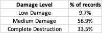
The data comes from drivendata.org but was originally sourced from the Nepal Earthquake Open Data Portal. It consists of 260,601 records with 38 features plus the target. The target is ternary: 1 = 'Low Damage', 2 = 'Medium Damage', and 3 = 'Complete Destruction'. The target is imbalanced: Low Damage = 9.7%, Medium Damage = 56.9%, and Complete Destruction = 33.5%.
A data dictionary is included in this repository, but the 38 features can broadly be divided into four categories: binary columns, categorical columns, integer columns, and geographical columns.
Binary columns: There are 22 binary (or 'flag') columns that use a 1 to designate that a building has that feature, or else a 0. The binary columns are divided into 'has_superstructure' and 'has_secondary_use' characteristics.
Categorical columns: There are eight categorical columns, with a total of 38 possibles values across all eight columns.
Integer columns: There are five integer columns.
Geographical columns: There are three geographical columns, 'geo_level_1_id', 'geo_level_2_id', and 'geo_level_3_id'. Level 1 is the broadest category, with only 30 unique values, followed by level 2 with 1427, and level 3 with 12567. We can assume that this means they represent descending levels of geographic range. So level 1 could be on the order of a city, level 2 a neighborhood, and level 3 a street. We aren't told what exactly they represent, but we at least surmise that they represent increasingly smaller geographical areas.
I first merge the values and labels dataframes on ‘building_id’ (a unique descriptor for each building), and then determine the target distribution. I divide the columns into four categories: eight categorical columns (with 38 unique features across all eight columns), 22 binary (flag) columns, five integer columns, and three geographical columns.
Categorical columns: These will be one hot encoded for modeling
Binary columns: Use a 1 to designate that a building has that feature, or else a 0. The binary columns are divided into 'has_superstructure' and 'has_secondary_use' characteristics.
Integer columns: I investigate the distribution of these features and can use log transformation and scaling for modeling.
Geographical columns: I investigate several possible encoders for these features, and settle on Target Encoding.
I investigate the correlations between the features and the target and note that there are weak correlations across the board. In fact the strongest (absolute) correlation is less than .3.
I also construct a baseline Random Forest model to investigate feature importances. I note that the geographical features are the top three, followed by age of the building. Some features have minimal importance, and I use various minimum thresholds to investigate dropping some features while modeling.
I build a dummy model that predicts the most frequent target, which yields a Micro Averaged F1 Score (see below) of .5689. I then proceed to build and evalute various models, using Logistic Regression, Random Forest, various boosting models, SVM, KNN, stacked models, and a Neural Network. This is further discussed in the 'Modeling Results' section.
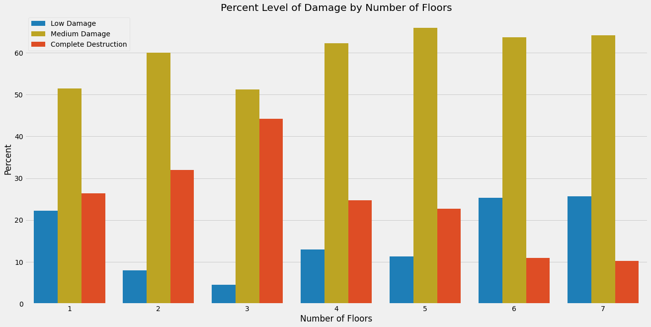
The target is encoded as follows: 1 = 'Low Damage', 2 = 'Medium Damage', 3 = 'Complete Destruction'. There is a target imbalance: 9.7% are 'Low Damage', 56.9% are 'Medium Damage', and 33.5% are 'Complete Destruction'.
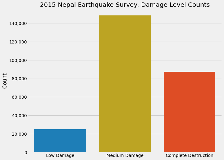
The age of the building has an effect on the damage level received. As the age of the building increases from new to around 30 years, the percentage of buildings that were completely destroyed increases, while the percentage of buildings receiving low damage decreases. Interestingly, after about 30 years of age, this effect wanes, and the levels of damage are roughly similar for buildings older than that.
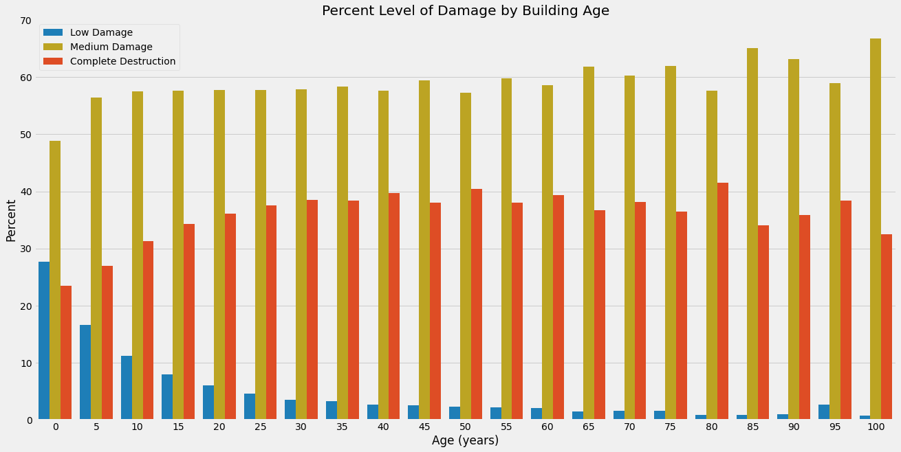
The damage received increases as the number of floors increases from one to three. Interestingly, though, as the number of floors increases above three, the level of damage decreases. We might surmise that this is because buildings taller than three floors are constructed with sturdier materials, a topic discussed under the next graphic.

This graphic shows the level of complete destruction based on the materials used for the building’s superstructure. Stone structures fare worst, followed by adobe mud and mud mortared brick. Timber and bamboo structures were in the middle. Better performing is cement mortared stone and non-engineered reinforced concrete (RC). Cement mortared brick performs very well. But by far the best structure for surviving the earthquake is engineered reinforced concrete.
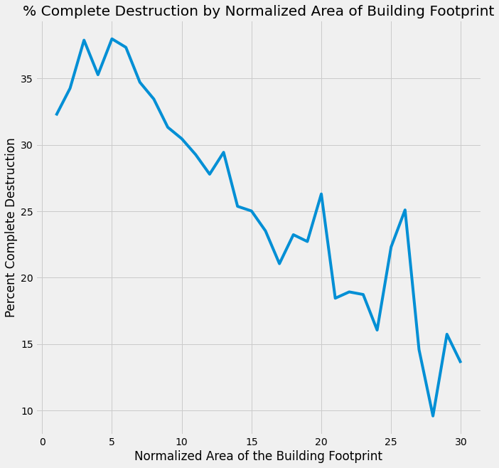
This graphic shows the percentage of buildings completely destroyed by the normalized area of the building footprint. These data suggest the as the footprint of the building increases, the percentage of buildings completely destroyed decreases. In other words, ‘stout’ buildings fare better than ‘skinny’ buildings.
The metric used for evaluating models is the Micro Averaged F1 Score. An F1 score reflects a blend of the precision and recall of the model, traditionally used on a binary classifier. Since there are three possible labels, I will use the Micro Averaged F1 Score variant.
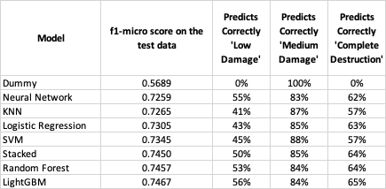
The modeling approach was to try many types of models and ensembles, to iterate and tune each one, and then to score the best version on the test set. The final f1-micro test scores are included in the table below:
After checking feature importances in a Random Forest model, I found that dropping certain less-important features not only improved runtimes but also f1-micro scores. I tested those dropped features on several models and the same held true.
I also discovered that resampling via SMOTE was not helpful on this dataset. In all cases where SMOTE was tried, including tree-based models, logistic regression, and neural networks, the cross-validated scores declined.
Proper encoding of the three geographical columns was paramount. These are high cardinality features, with ‘geo_level_3_id' having 12,567 possible values. They represent the location of each of the buildings. One approach tried was to OHE these features and then use PCA to reduce dimensionality. But the runtimes were expensive and the scores lackluster, so I abandoned this approach. In notebook 10, however, I try several different categorical encoders including Target, LeaveOneOut, Hashing, and JamesStein. Target encoding yields the best results and that is the approach I used with all of the models. I was able to ‘tune’ the Target Encoder to squeeze a slightly better performance out of the lightGBM model.
The models all scored similarly: there is, in fact, only about a 0.02 score difference between the best and worst performing models. There are, however, significant differences in runtime. The neural networks, logistic regression, and lightGBM all fit in less than a minute on my machine, while the stacked model takes over an hour and SVM takes many hours.
There is also some difference in the ability of the models to correctly predict each of the labels. All of the models do well predicting ‘medium damage’, the most frequent label (predicting in the range of 83%-87%), less so with with ‘complete destruction’ (57%-65%), and even less so with the least frequent label, ‘low damage’ (41%-56%).
Given it’s f1-micro score, runtime, and ability to predict the less frequent labels, the model that shines is lightGBM. It was not only the best and fastest boosted model, beating XGBoost, but also the best model overall. An untuned five-fold cross-validation was completed in under a minute while achieving the highest f1-micro score on the test data. It also was the best at correctly predicting ‘low damage’ and ‘complete destruction’. The Random Forest model scored and predicted similarly, though at a runtime many multiples of lightGBM.
Though it’s f1-micro score is lower, the neural network also did well at correctly predicting the less frequent labels. And, given its speed, this model also deserves mention.
Please review my full analysis in different notebooks: Data Exploration Notebook, Random Forest Models Notebook, PCA Notebook, Logistic Regression Notebook, Boosters Notebook, SVM Notebook, KNN Notebook, Stacking Notebook, Neural Network Notebook, and the Encoder Notebook or the Presentation.
├── data                                  <- Sourced from drivendata.org
├── images                                <- Images that were used in the presentation and notebooks

├── 01_Data_Exploration.ipynb             <- EDA Notebook
├── 02_Random_Forest.ipynb                <- Random Forest Models
├── 03_PCA.ipynb                          <- Principal Component Analysis
├── 04_LogisticRegression.ipynb           <- Logistic Regression Models
├── 05_Boosters.ipynb                     <- Boosted Models
├── 06_SVM.ipynb                          <- Support Vector Machines Models
├── 07_KNN.ipynb                          <- K-Nearest Neighbors Models
├── 08_Stacking.ipynb                     <- Stacked Model
├── 09_Neural Network.ipynb               <- Neural Network Model
├── 10_Encoders.ipynb                     <- Testing Various Encoders
├── gitignore                             <- Python files to ignore
├── Presentation.pdf                      <- PDF of the project presentation
├── Data_Dictionary.md                    <- Data Dictionary
└── README.md                             <- The README.md