Open-source Python toolkit for parametric modeling, simulation, visualization, and multidisciplinary design optimization of axial-flux permanent-magnet motors.
![]()

Full documentation, including theory derivations, the API reference, and executed example notebooks: jman4162.github.io/axfluxmdo
axfluxmdo is a design-exploration layer for axial-flux machines. It does not replace
expert designers or high-fidelity FEA; it supplies the fast, validated models around
them: parametric geometry, closed-form and 2.5D physics, open-source solver automation,
and Pareto-front and Bayesian optimization. The goal is to make design tradeoffs
explicit and quantitative early, before committing to detailed simulation or hardware.
The package covers five layers: an analytical workbench (energy-consistent torque/back-EMF/loss/thermal model with named constraints), a 2.5D annular slice model (radius-resolved fields, manufacturing imperfections, torque ripple, axial force, efficiency maps), a multi-objective optimization layer (pymoo Pareto fronts, OpenMDAO integration, sensitivities), external solver hooks (Gmsh mesh export and a GetDP magnetostatics pipeline with residual analysis), and Gaussian-process surrogates with Bayesian optimization for expensive objectives. A design evaluation takes microseconds, so a full Pareto study completes in seconds, and the analytical layer's error budget is quantified against open-source FEA rather than assumed.
pip install axfluxmdo                  # core (analytical + annular models, 2D viz)
pip install "axfluxmdo[opt]"           # + pymoo / OpenMDAO / scikit-learn optimization
pip install "axfluxmdo[fea]"           # + gmsh mesh export (GetDP is a separate binary)
pip install "axfluxmdo[viz3d]"         # + PyVista 3D rendering/animations
For development:
git clone https://github.com/jman4162/axfluxmdo.git
cd axfluxmdo
pip install -e ".[dev,opt,fea,viz3d]"from axfluxmdo import AxialFluxMotor, OperatingPoint
from axfluxmdo.models import AnalyticalModel
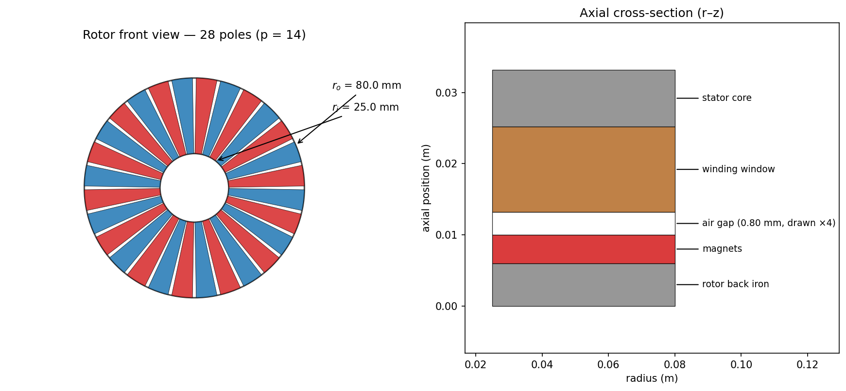
from axfluxmdo.viz import plot_geometry
motor = AxialFluxMotor(
outer_radius=0.08, # m
inner_radius=0.025, # m
air_gap=0.0008, # m
pole_pairs=14,
phases=3,
turns_per_phase=24,
fill_factor=0.45,
magnet_thickness=0.004, # m
back_iron_thickness=0.006, # m
)
op = OperatingPoint(speed_rpm=500, current_rms=25, dc_bus_voltage=48)
result = AnalyticalModel().evaluate(motor, op)
print(result)
plot_geometry(motor, show=True)AnalyticalResult
torque: 8.629 N·m
torque density: 2.364 N·m/kg
back-EMF (rms): 6.02 V/phase
elec frequency: 116.7 Hz
air-gap B: 1.016 T
current density: 4.04 A/mm²
copper loss: 20.0 W
core loss: 0.91 W
efficiency: 0.9557
winding temp: 49.6 °C
mass: 3.651 kg
constraints:
winding_temp_c: 49.57 <= 140 [OK, margin +64.6%]
electrical_frequency_hz: 116.7 <= 1000 [OK, margin +88.3%]
current_density_a_mm2: 4.042 <= 10 [OK, margin +59.6%]
line_voltage_v: 10.9 <= 33.94 [OK, margin +67.9%]
core_flux_density_t: 0.6696 <= 1.6 [OK, margin +58.2%]
magnet_temp_c: 65 <= 80 [OK, margin +18.8%]
Axial-flux machines suit robot joints for two structural reasons: the pancake aspect ratio packages well inside joint envelopes, and high pole counts work naturally at the low speeds and high torques of direct-drive or low-ratio actuators. Several parts of the package map directly onto actuator development work:
- Sizing at the duty point. Every evaluation reports thermal, voltage, current-density, and saturation margins, so a candidate joint motor can be screened against its continuous and peak torque requirements before any FEA.
- Manufacturing sensitivity. Air-gap error, rotor coning, and runout are first-class design variables. Their effects on torque ripple and axial bearing load are computed per design; both matter for joint control bandwidth and encoder integrity.
- Duty-cycle energy. Constraint-aware efficiency maps over the joint's speed–torque envelope support trajectory-level energy estimates.
- Actuator tradeoff studies. Pareto fronts over torque density, efficiency, and mass under joint constraints; Bayesian optimization when the objective involves an FEA solve or test-stand data.
- System co-design. The OpenMDAO component lets the motor model participate in arm-level optimization together with gearbox, inverter, and structural models.
The standard caveats in Model fidelity & known limitations apply with extra force for actuators: the model is single-gap, ripple is a proxy rather than a waveform, and designs should be validated against FEA and hardware before commitment.
from axfluxmdo.sweeps import sweep_pole_pairs

sweep = sweep_pole_pairs(motor, op, pole_pairs=range(4, 21, 2))
sweep.plot(show=True)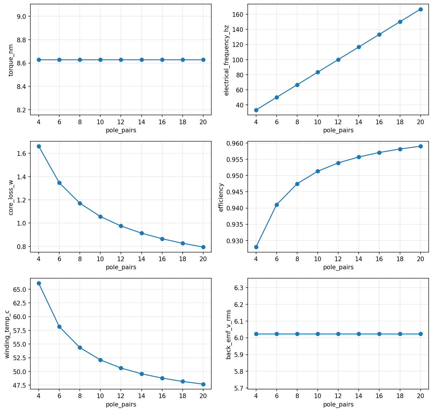
At fixed air-gap field and electrical loading, torque is independent of pole count. The flat curve is correct physics, not a model artifact: flux per pole falls as 1/p while the pole count rises as p, and the two cancel exactly in the torque expression. The common intuition that more poles means more torque comes from torque density: high pole counts permit thinner yokes, and resizing the iron accordingly raises torque per kilogram by several times while torque itself stays constant. In this fixed-geometry sweep the real tradeoff is yoke saturation at low p (p = 4 is infeasible here because the fixed stator core would need to carry 2.3 T) against electrical frequency, switching burden, and ripple at high p. The pole-pair explainer in the docs works through the algebra and both sweeps.
import dataclasses
from axfluxmdo import GapImperfections
from axfluxmdo.models import AnnularModel, compute_efficiency_map
imperfect = dataclasses.replace(
motor,
tolerances=GapImperfections(gap_offset_m=1e-4, coning_m=2e-4, runout_m=3e-4),
magnet_shape="rectangular",
)
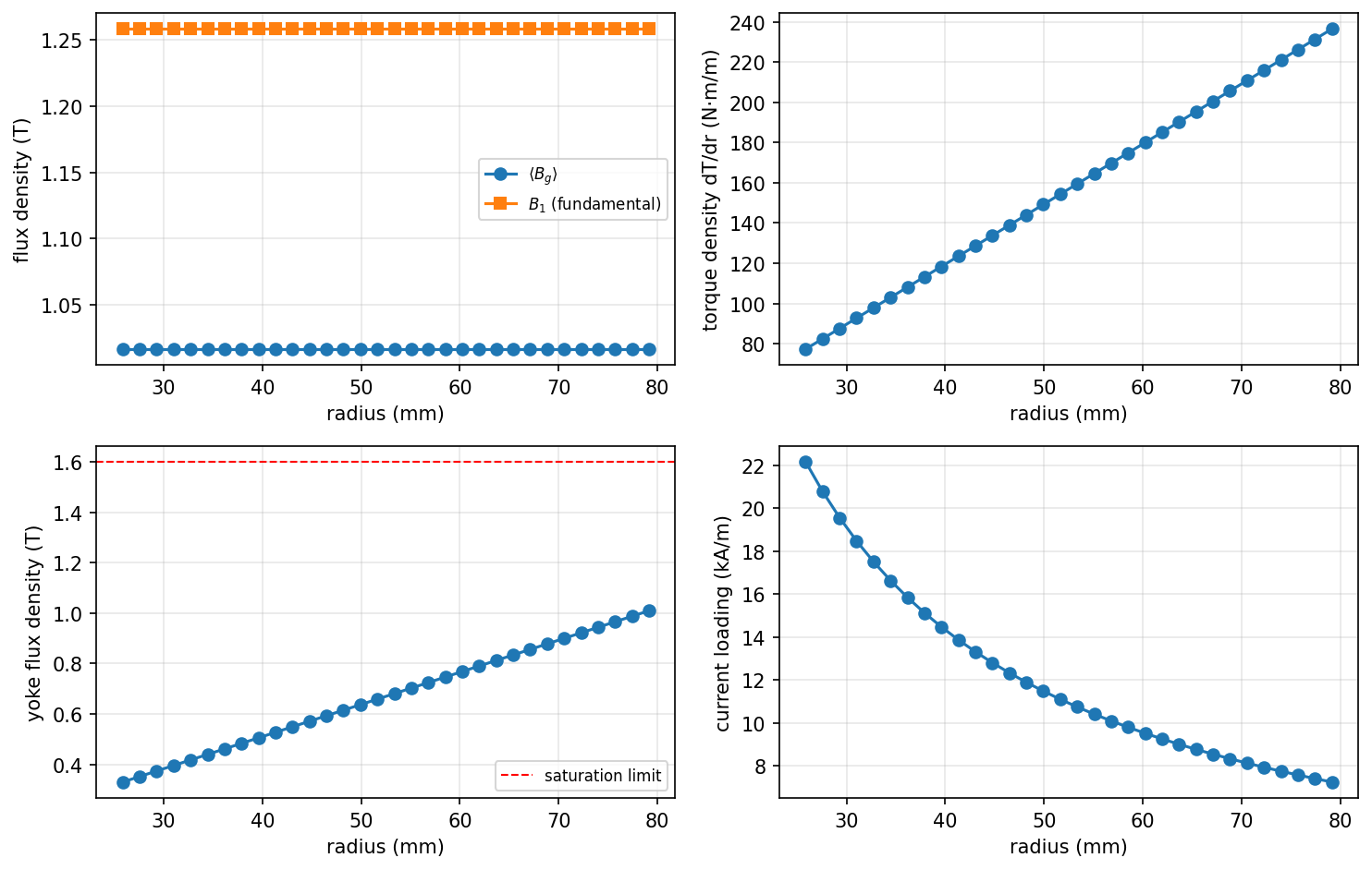
result = AnnularModel(n_slices=32).evaluate(imperfect, op)
print(result.torque_ripple_proxy, result.axial_force_n)
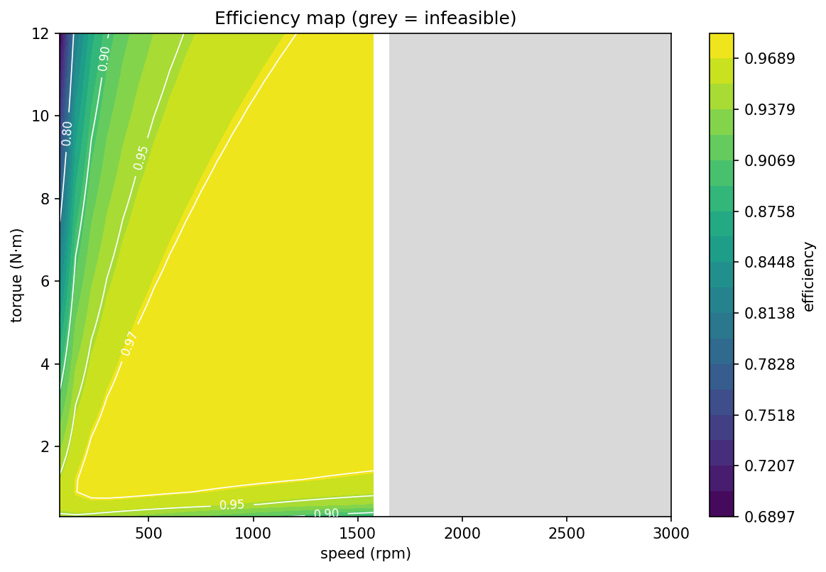
emap = compute_efficiency_map(motor, op, max_speed_rpm=3000, max_torque_nm=12)
emap.plot(show=True)The disk machine is split into radial annuli. Torque and back-EMF derive from the same summed flux linkage, so for a perfect machine the annular model agrees with the analytical layer to machine precision (pinned by tests). Added fidelity appears only where physics is genuinely radius-dependent:
- Yoke saturation binds at the outer radius, where the pole pitch is widest. The mean-radius proxy of Layer 1 underestimates it.
- Manufacturing imperfections: uniform gap error, rotor coning, and runout. The runout average is analytic; because the load line is convex in the gap, mean torque rises slightly with runout, and the real penalties are the 1/rev ripple proxy and the axial-force modulation.
- Constraint-aware efficiency maps over the speed–torque plane, with the binding constraint recorded for every infeasible cell.
Requires the optimization extra: pip install "axfluxmdo[opt]" (pymoo + OpenMDAO).
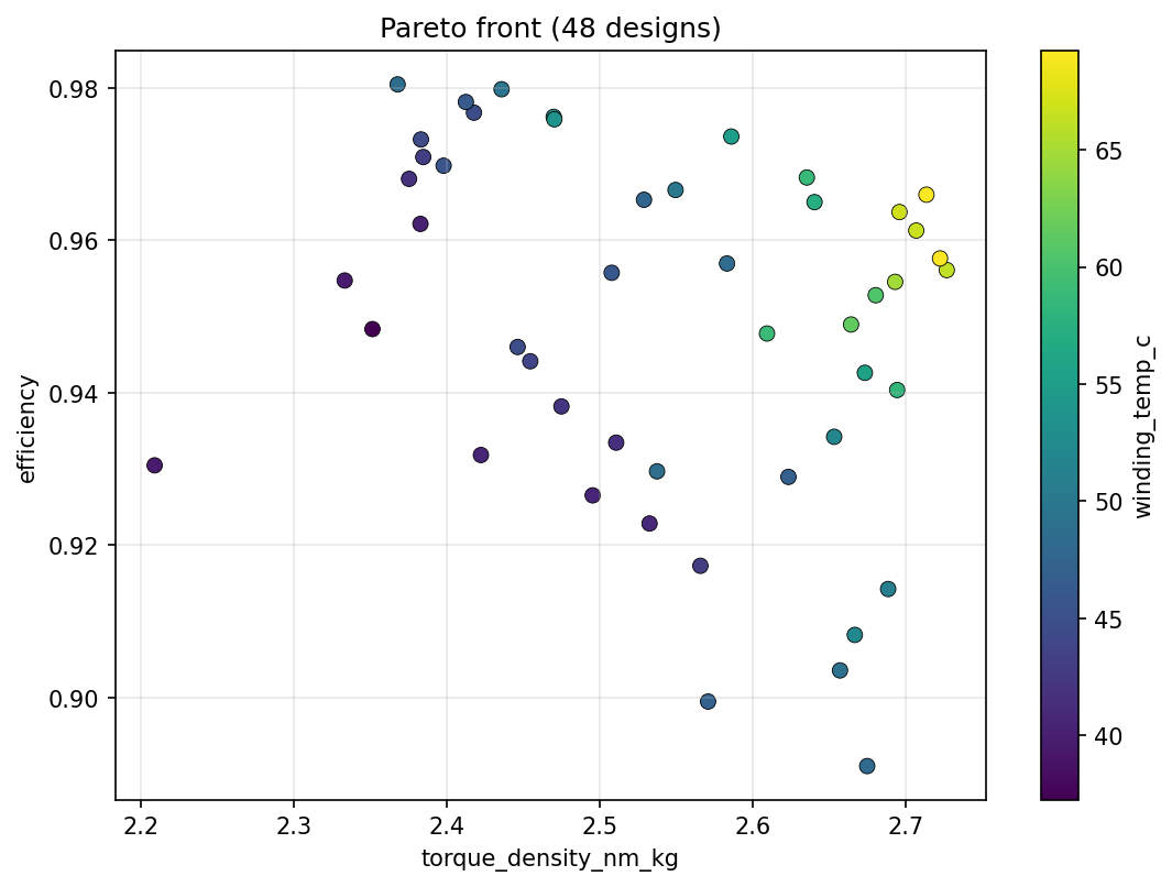
from axfluxmdo.optimize import optimize_pareto
from axfluxmdo.viz import plot_pareto

study = optimize_pareto(
    motor,
    op,
    variables={
        "outer_radius": (0.05, 0.12),
        "pole_pairs": [8, 10, 12, 14, 16, 18, 20],
        "air_gap": (0.0005, 0.0015),
        "fill_factor": (0.30, 0.60),
    },
    objectives=["maximize_torque_density", "maximize_efficiency", "minimize_mass"],
    constraints=["winding_temp_c < 140", "electrical_frequency_hz < 1000"],
)

plot_pareto(study, x="torque_density", y="efficiency", color="winding_temp_c", show=True)
Mixed continuous/discrete variables run through pymoo's MixedVariableGA. The model's
built-in limits (thermal, voltage, current density, saturation, magnet temperature) are
enforced in addition to the user constraint strings, so every returned design is
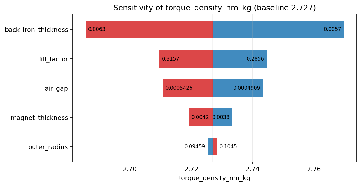
feasible. One-at-a-time sensitivities (compute_sensitivities + plot_tornado) rank
the variables that move a chosen design, and an OpenMDAO ExplicitComponent wrapper
supports gradient-based refinement and larger coupled MDO groups.
from axfluxmdo.solvers import solve_open_circuit # needs getdp on PATH
from axfluxmdo.validation import compare_open_circuit, measured_carter_factor
slotless = solve_open_circuit(motor, magnet_temp_c=65.0) # gmsh -> GetDP -> parsed field
slotted = solve_open_circuit(motor, slotted=True, magnet_temp_c=65.0)
print(compare_open_circuit(motor, slotless, magnet_temp_c=65.0))
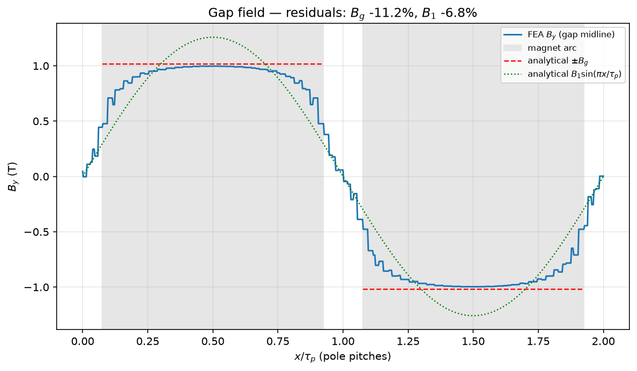
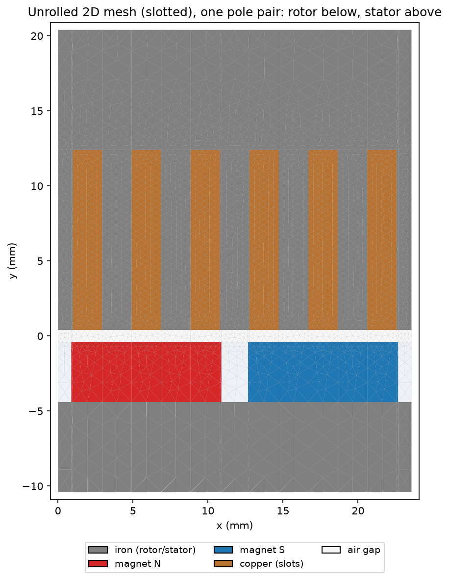
print(measured_carter_factor(slotless, slotted, motor))The annulus is unrolled at the mean radius into a 2D planar magnetostatics problem
(one pole pair, periodic), meshed by Gmsh (pip install "axfluxmdo[fea]") and solved
open-circuit by GetDP. GetDP is an external binary; tests and examples fall back to
committed golden results without it. The FEA uses the same recoil-line magnet model as
the analytical load line, so residuals isolate geometric effects the 1D circuit cannot
represent. Measured on the reference motor (GetDP 3.5.0):
- The load line overestimates the gap field. FEA's under-magnet mean is 11.2% lower than B_g and the fundamental is 6.8% lower than B₁, due to inter-magnet leakage and fringing.
- Slotting reduces the field a further 7.6%, corresponding to a measured Carter factor
k_C = 1.44. Feeding that value back through
carter_factor=reproduces the FEA slotless/slotted ratio to four decimal places.
A 3D annular-sector mesh export (export_3d_sector) is included for downstream
tooling. Elmer integration is deferred.
from axfluxmdo.optimize import bayesian_optimize
study = bayesian_optimize(
motor,
op,
variables={
"outer_radius": (0.05, 0.12),
"air_gap": (0.0005, 0.0015),
"fill_factor": (0.30, 0.60),
"pole_pairs": [8, 10, 12, 14, 16, 18, 20],
},
objective="maximize_torque_density",
constraints=["winding_temp_c < 140", "electrical_frequency_hz < 1000"],
n_initial=10,
n_iterations=25,
seed=42,
)
print(study.summary())
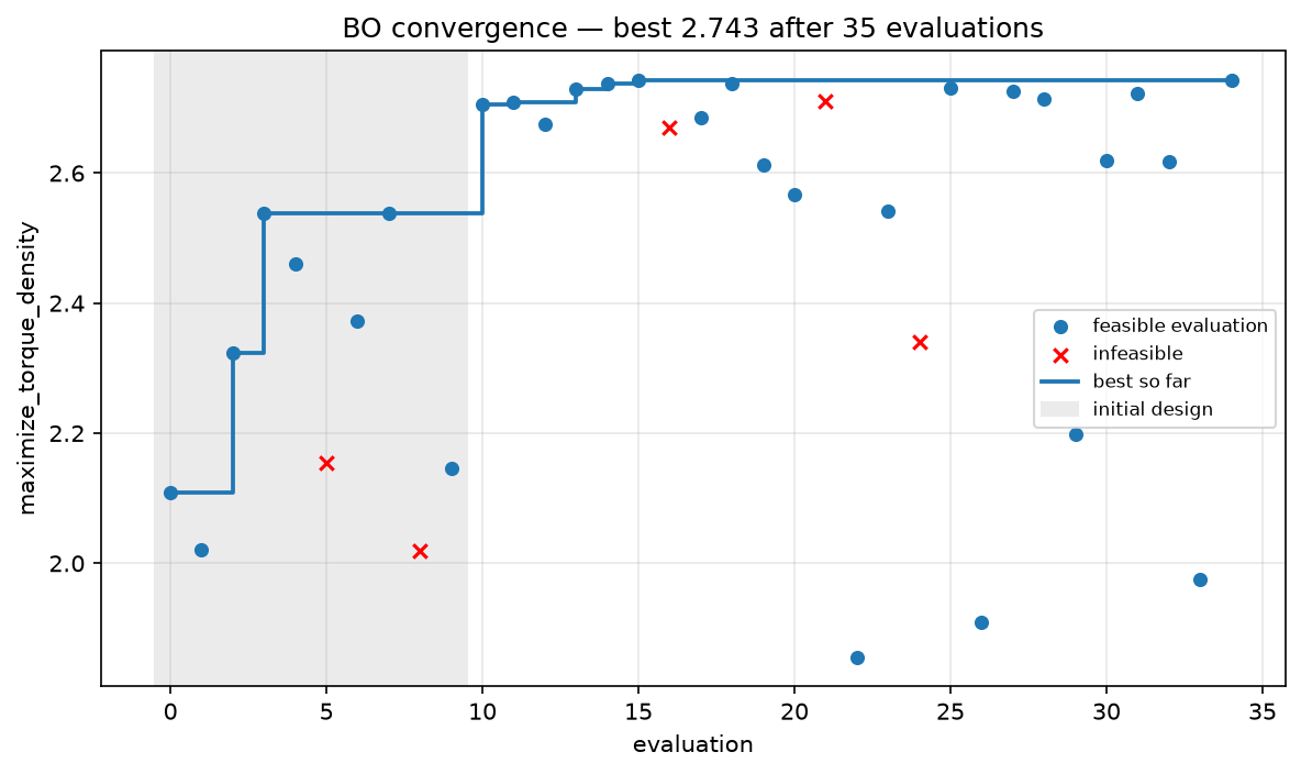
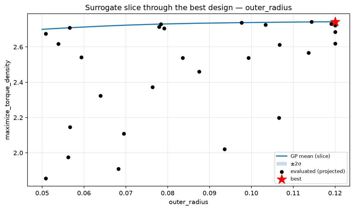
print(study.recommend(k=3)) # ranked by surrogate mean minus uncertaintyA Gaussian-process surrogate (ARD Matérn, scikit-learn) with expected-improvement
acquisition reaches the genetic algorithm's torque-density optimum in 35 evaluations
instead of roughly 1200. That matters when each evaluation is an FEA solve or a dyno
run. An expensive_fn hook plugs any costly objective into the loop, every evaluation
is recorded in a persistable DesignDataset (JSON Lines), and recommendations are
ranked by the surrogate's pessimistic estimate so that poorly explored regions of the
design space are not selected on optimism.
from axfluxmdo.viz import plot_motor_3d, animate_rotation, animate_exploded
plot_motor_3d(motor, show=True) # interactive cutaway view
animate_rotation(motor, "rotation.gif") # rotor spinning over the stator
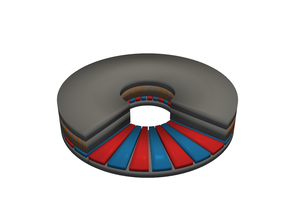
animate_exploded(motor, "exploded.gif") # assembly exploding/reassemblingThe parametric motor renders as a 3D assembly via PyVista
(pip install "axfluxmdo[viz3d]"): rotor back iron, alternating N/S magnets, the
slotted stator with copper coils, and the yoke. Every solid is built from the same
AxialFluxMotor dimensions the physics models use; mesh volumes match the analytic
volume properties to better than 0.1% (tested).

The base layer computes the magnet load-line air-gap flux density (with
temperature-derated remanence and an optional measured carter_factor), then derives
torque and back-EMF from a single flux linkage so the power balance m·E·I = T·ω
holds to machine precision (test-enforced). Losses are DC copper with
resistance–temperature coupling and two-term Steinmetz core loss with
datasheet-pinned M-19 coefficients. The thermal model is a closed-form lumped RC with
thermal-runaway detection. Six named constraints (winding temperature, electrical
frequency, current density, inverter voltage, yoke saturation, magnet temperature)
report normalized margins on every evaluation. The
analytical model guide
derives each equation.
pip install -e ".[dev]"
pytest                       # full suite
ruff check . && ruff format --check .All five SPEC phases are shipped.
| Phase | Scope | Status |
|---|---|---|
| 1 | Analytical workbench: parametric motor, torque/EMF/losses/thermal RC, constraints, pole-pair sweep, geometry viz | ✅ |
| 2 | 2.5D annular slice model: radius-dependent flux/loading/losses, air-gap & runout sensitivity, efficiency maps | ✅ |
| 3 | MDO: OpenMDAO components, pymoo Pareto optimization, sensitivity analysis | ✅ |
| 4 | External solver integration: Gmsh export, GetDP pipeline, sim-to-analytical residuals (Elmer deferred) | ✅ |
| 5 | Surrogates & Bayesian optimization for expensive design loops | ✅ |
The fast layers are deliberately simple. Know what they leave out before trusting absolute numbers; each item is also documented at the relevant docstring.
- Single-gap topology (one rotor, one stator). Real axial-flux machines are often
double-gap (TORUS/YASA/AFIR). The single-sided rotor carries a large unbalanced
axial pull, reported by
AnnularResult.axial_force_n(about 5–6 kN for the reference motor), and the bearings must take it. - The 1D load line is an upper bound on the gap field. FEA validation measured 11%
low on the under-magnet mean and 7% low on the fundamental, plus a Carter factor
k_C = 1.44 for the slotted stator. Both models accept
carter_factor=to fold a measured correction back in. - No magnetic saturation: torque is linear in current. The yoke-flux and current-density constraints are the guards.
- The voltage constraint neglects inductive drop (I·X_L), which is optimistic at high electrical frequency with tight bus margins.
- Magnet temperature is fixed at ambient + 40 °C, not coupled to the solved winding temperature.
- The thermal model is a single lumped RC with constant resistance and no speed-dependent cooling; 50% of core loss is assigned to the winding node.
- Losses omitted: AC copper (skin/proximity), magnet eddy currents, PWM harmonics. Mechanical loss defaults to zero and is parameterizable.
- No custom FEM solver; geometry/mesh export targets open tools (Gmsh, GetDP/ONELAB, Elmer).
- No full transient 3D EM FEA, CFD, structural, or inverter-switching simulation in v1.
- No dependencies on proprietary tools (Motor-CAD, Ansys Maxwell, COMSOL).
- Torque density is never optimized alone; thermal headroom, ripple, controllability, and manufacturability are co-equal objectives.
If you use axfluxmdo in academic work, please cite it:
@software{hodge_axfluxmdo_2026,
  author  = {Hodge, John},
  title   = {axfluxmdo: Parametric modeling, simulation, and multidisciplinary
             design optimization of axial-flux permanent-magnet motors},
  year    = {2026},
  version = {0.7.0},
  url     = {https://github.com/jman4162/axfluxmdo},
  note    = {Documentation: https://jman4162.github.io/axfluxmdo/}
}