cQEDraw

cQEDraw draws and analyzes superconducting circuit graphs for Black Box Quantization workflows. It generates sparse capacitance and inverse-inductance matrix snippets and can run in-browser modal analysis for supported circuits. The browser app is the primary interface; new feature work and routine refactors target the web app. The standalone Tkinter desktop app remains available as a legacy maintenance-only interface.

Open the web editor: https://cqedraw.org/

It is the companion GUI matrix-builder for sccircuits: use the app to draw the linear circuit, then paste the generated matrices into a Python analysis that constructs sccircuits.BBQ objects. The app remains installable on its own because it is a launched desktop-style tool, not an imported library API.

What cQEDraw Helps With

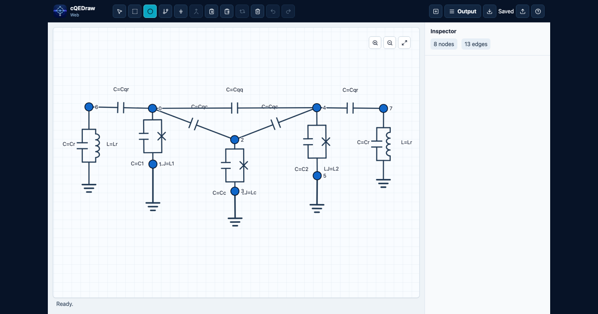
• Draw superconducting circuit graphs directly in the browser.
• Generate sparse SciPy capacitance and inverse-inductance matrix snippets.
• Preserve Josephson-junction branch metadata for Black Box Quantization workflows.
• Run in-browser modal analysis for supported circuits without local Python setup.
• Export analysis tables as CSV for downstream notebooks and scripts.

Share cQEDraw

• Canonical URL: https://cqedraw.org/
• Tagline: Draw and analyze superconducting circuit graphs for Black Box Quantization workflows.
• Social preview image: https://cqedraw.org/social-card.png
• Reusable launch copy: docs/launch-copy.md

v0.2.0 Milestone Scope

v0.2.0 is the first web-analysis milestone. It supports drawing circuit graphs, copying sparse Python matrix snippets, preserving Josephson junction branch metadata, running in-browser sccircuits.BBQ modal analysis, plotting mode frequencies and Josephson phase zero-point fluctuations, sweeping parameter values with sliders, and exporting the current analysis table as CSV.

The supported analysis scope is intentionally limited:

• Modal analysis assumes the evaluated capacitance and inverse-inductance matrices are well-posed for the generalized eigenvalue problem.
• cQEDraw does not yet model external loop fluxes.
• cQEDraw does not silently reduce, eliminate, or classify free, frozen, constrained, periodic, or extended variables.
• Physical graph-to-Hamiltonian reduction is planned for sccircuits; cQEDraw will preserve and export graph metadata needed by that later layer.

This boundary follows the broader computer-aided circuit quantization problem discussed in Computer-aided quantization and numerical analysis of superconducting circuits. Time-dependent external-flux and microwave-drive Hamiltonians are also outside this milestone; see Systematic Construction of Time-Dependent Hamiltonians for Microwave-Driven Josephson Circuits.

The current matrix snippet workflow remains useful outside this scope: advanced users can copy the sparse matrices and handle reductions or external fluxes in their own Python analysis.

Install And Open

Web App

This is the lowest-friction path and the actively maintained interface:

1. Open https://cqedraw.org/
2. Use cQEDraw in the browser.
3. Install it from the browser menu if you want it in the ChromeOS or desktop launcher.

The web app runs the same Python/SymPy output logic in the browser through Pyodide. It does not require Python, Pixi, or a terminal on the user's machine. The GitHub Pages project URL remains available as a fallback during the custom domain rollout.

macOS And Windows Legacy Desktop Builds

This path remains available for users who prefer a local desktop app, but the desktop app is legacy maintenance-only. Use the web app for the actively maintained interface, including new analysis and plotting features.

1. Open the latest release: https://github.com/joanjcaceres/cqedraw/releases/latest
2. Download cQEDraw-macOS.zip on macOS or cQEDraw-Windows.zip on Windows.
3. Unzip the downloaded file.
4. Open cQEDraw.app on macOS or cQEDraw.exe on Windows.

The desktop downloads include Python plus the required NumPy, SciPy, and SymPy runtime dependencies. They are unsigned beta builds, so macOS or Windows may show a security warning the first time you open them.

Linux Or Python Install

Use this path on Linux, or if you prefer to manage Python applications from the terminal. It requires Python 3.11 or newer and either pipx or pip. It does not require Pixi.

Run without a permanent install using pipx:

pipx run --spec git+https://github.com/joanjcaceres/cqedraw.git cqedraw

Install with pip:

python -m pip install "cqedraw @ git+https://github.com/joanjcaceres/cqedraw.git"
cqedraw

Install together with SCCircuits for analysis examples:

python -m pip install "cqedraw[sccircuits] @ git+https://github.com/joanjcaceres/cqedraw.git"

For Python installs only, Tkinter must be available in your Python installation. Tkinter is part of the Python standard library, but some Linux distributions ship it separately. If the app fails with ModuleNotFoundError: tkinter, install your platform's Tk package, for example python3-tk on Debian/Ubuntu.

You can also launch a Python install as a module:

python -m cqedraw

To verify a Python install without opening the GUI:

cqedraw --version

Local Development

Use this path only if you want to modify cQEDraw or run the test suite.

git clone https://github.com/joanjcaceres/cqedraw.git
cd cqedraw
python -m pip install -e ".[dev]"
pytest

For the web app:

cd web
npm install
npm run dev

Basic Workflow

Use the toolbar or keyboard shortcuts to create nodes, edges, and ground connections. Edge dialogs accept numeric values or SymPy-compatible symbolic expressions for capacitance, linear inductance, and Josephson inductance.

Projects can be saved and loaded as JSON files from the GUI. Use Copy matrices to copy generated Python code for the current capacitance matrix and inverse-inductance matrix. The generated snippet returns sparse SciPy CSR matrices so large circuits do not allocate dense zero-filled arrays. Canvas node labels show the matrix row/column index used in generated output; the editable node name is preserved as metadata in the inspector and snippet node maps.

The web analysis panel can accept numeric energy values instead of component values when a parameter is used directly as a single capacitance, linear inductance, or Josephson inductance. Energy entries use GHz for E/h and are converted before modal analysis as C = e^2 / (2 h E_C), L = phi0^2 / (h E_L), and LJ = phi0^2 / (h E_J), where the entered GHz values are first converted to Hz and phi0 = hbar / (2e). This is an analysis UI convenience only: saved projects and copied Python snippets still use the capacitance and inductance symbols drawn in the circuit.

Using With SCCircuits

The copied snippet defines circuit_matrices, capacitance_matrix, inverse_inductance_matrix, josephson_branches, MATRIX_NODES, and NODE_INDEX_MAP. Paste that snippet into your analysis script or notebook, then pass the parameter values as a mapping:

from sccircuits import BBQ

# Paste the snippet copied from cQEDraw above this line.
# Replace these names and values with the symbols used in your drawing.
capacitance_matrix, inverse_inductance_matrix = circuit_matrices(
    {"Cj": 40e-15, "Cg": 2e-15, "Lj": 1.23e-9}
)
junctions = josephson_branches({"Cj": 40e-15, "Cg": 2e-15, "Lj": 1.23e-9})
branch = junctions[0]
nonlinear_branches = (
    (branch["phase_positive_index"],)
    if branch["phase_negative_index"] is None
    else (branch["phase_negative_index"], branch["phase_positive_index"])
)

bbq = BBQ(
    capacitance_matrix,
    inverse_inductance_matrix,
    nonlinear_branches=nonlinear_branches,
)

print("Project node to matrix index:", NODE_INDEX_MAP)
print("Linear mode frequencies (GHz):", bbq.frequencies_ghz)
print("Phase ZPF:", bbq.branch_phase_zpfs)

For direct generalized eigenvalue analysis, keep the matrices sparse:

import numpy as np
from scipy.sparse.linalg import eigsh

# Paste the snippet copied from cQEDraw above this line.
capacitance_matrix, inverse_inductance_matrix = circuit_matrices(
    {"Cj": 40e-15, "Cg": 2e-15, "Lj": 1.23e-9}
)

omega_squared, modes = eigsh(
    inverse_inductance_matrix,
    k=4,
    M=capacitance_matrix,
    sigma=0.0,
    which="LM",
)
frequencies_hz = np.sqrt(np.maximum(omega_squared, 0.0)) / (2 * np.pi)

In the web app, after generating a circuit, enter numeric parameter values in the Output panel. Analysis runs automatically when the required values are complete. The app uses sccircuits.BBQ to display mode frequencies and, when Josephson junctions are present, one phase-ZPF row per junction. In the browser build, the BBQ class is loaded on demand from the sccircuits repository; in Python environments, install cQEDraw with the sccircuits extra to use the same analysis path locally.

Click Export CSV to download the frequency and Josephson-junction zero-point fluctuation table for use in a separate Python script:

import pandas as pd

table = pd.read_csv("cqedraw-analysis-table.csv")

The CSV is intentionally just the table. The first column is frequency_ghz; each additional column is the phase ZPF for one Josephson junction, such as phase_zpf_edge_7. It leaves the project, symbolic matrices, and dense matrices in the regular project file and copied Python snippet.

If you only need to draw circuits and copy matrix snippets, sccircuits is not required. Install the optional sccircuits extra when you want the analysis package available in the same environment.

Development

python -m pip install -e ".[dev]"
pytest

Regenerate icon assets after replacing assets/icon-source.png:

python scripts/generate_icons.py

Build local Python distributions:

python -m build

Create a release by pushing a version tag:

git tag v0.2.0
git push origin v0.2.0

The release workflow builds Python distributions plus macOS and Windows unsigned beta artifacts, then uploads them to GitHub Releases. PyPI publishing is intentionally disabled for the first beta release.

The tests cover matrix assembly, generated snippet behavior, CLI version handling, and node merge logic without opening the Tkinter window.

Run the web checks from web/:

npm run typecheck
npm test
npm run build
npm run test:e2e

The web app is deployed to GitHub Pages by .github/workflows/pages.yml after changes land on main. The repository's Pages source must be set to GitHub Actions once in the GitHub settings.

Support And CI Policy

The web app is the primary product surface. New UI features, analysis UX work, and maintainability refactors should target web/ unless a change is needed to preserve shared matrix-output behavior.

The Python desktop app is legacy maintenance-only. Keep it loadable and avoid breaking existing Python tests, but do not start broad desktop refactors for new web functionality. Shared Python modules such as cqedraw/core.py and cqedraw/web_bridge.py still matter because the web app uses them through Pyodide.

Pull-request CI is path-aware:

• Web changes run the web typecheck, unit tests, build, and Playwright suite.
• Python, desktop, packaging, or Python-test changes run the Python test matrix.
• Shared Python output changes also run the web checks because they can affect browser-generated matrices.
• Documentation-only PRs may run only the CI policy summary.
• Pushes to main run both Python and web checks.