title	Cyclistic bike-share analysis case study
output	html_document pdf_document default default

Data analysis method:

Ask ->Prepare -> Process -> Analyze -> Share -> Act

Overview

In this blog is my process and perform to solve the problem of the case study: Cyclists bike-share. The main object of this case is “how to convert casual riders (customers who purchase full-day passes or single rides) to member riders (customers who purchase annual memberships). Particularly, the company wants to increase the number of their annual membership. You can find the full details of the case study here link

Ask

As Junior Data Analyst, the questions that I need to anwser using the given dataset are:

• How do annual members and casual riders use Cyclistic bikes differently?
• Why would casual riders buy Cyclistic annual memberships?
• How can Cyclistic use digital media to influence casual riders to become members?

Prepare

In this stage, I prepare the data by obtaining the data sets and storing it.The data sets was given as a monthly data in zip file. I downloaded the last 11 months of trip data which mean I downloaded 11 zip files. you can find the name of the files name was downloaded below:

• 202101-divvy-tripdata.zip
• 202102-divvy-tripdata.zip
• 202103-divvy-tripdata.zip
• 202104-divvy-tripdata.zip
• 202105-divvy-tripdata.zip
• 202106-divvy-tripdata.zip
• 202107-divvy-tripdata.zip
• 202108-divvy-tripdata.zip
• 202109-divvy-tripdata.zip
• 202110-divvy-tripdata.zip
• 202111-divvy-tripdata.zip

Process

In this phase, I processed the data and prepared it for our next phase where we will uncover answers to our questions. I used DB Browser for SQLite for this step since the dataset is too large to merge and operate (around 5 million raws). "DB Browser for SQLite (DB4S) is a high quality, visual, open source tool to create, design, and edit database files compatible with SQLite.

At first, I imported all the 11 .csv files with DB Browser on my computer and I modified files name to the month short name. Then, I used Union function to combine the result of more SELECT statement, but it took too much time and crached after some point. I managed to merge the csv files without running any code in DB Browser for SQLite using into one large data-set and exported to my device.

Secondly, using Rstudio, I installed all necessary packages using install.packages()

install.packages("tidyverse")

Next, downloaded all the packages that are on essential part for my workflow for the analysis.

library(ggplot2)
library(tidyr)
library(dplyr)
library(readr)
library(readxl)

The chunk code below is for importing the merged dataset

bikeshare2021 <- read.csv("/Users/othmanalamoudi/Desktop/R-project/BikeShare_2021.csv")

let's observe the number of rows & columns:

nrow(bikeshare2021) 
ncol(bikeshare2021)

As you can see, our data set became very large with more than 5 millions row and 13 columns. Now let's take a peek to the data set using head function, which shows only the fist rows - Side note: Iused knitr package to make the table looks pretty.

library(knitr)
knitr::kable(head(bikeshare2021),"pipe")

We have 13 columns and we can infer their content:

• ride_id: unique Id for each trip taken
• rideable_type: he type of a bike
• started_at: date and time of the start time
• ended_at: date and time of the end time
• start_station_name: name of the starting station
• start_station_id: id of the starting station
• end_station_name: Nnme of the ending station
• end_station_id: id of the ending station
• start_lat: latitude of the starting point
• start_lng: longitude of the starting point
• end_lat: latitude of the ending point
• end_lng: longitude of the ending point
• member_casual: the membership status (member, casual)

Looking at the column above, I figured I will be able to generate the distance travel where I will calculate the distance for each trip in meter using those four columns: start_lat, start_lng, end_lat and end_lng. For this I will need to use *Harversine formula where I it will calculates the distance in meter. ( I had to google this to figure it out)

I started with creating two data frames:

• Point 1: start_lat , end_lng
• point 2: end_lat, start_lng

point1 <- select(bikeshare2021, start_lat, end_lng)
point2 <- select(bikeshare2021, end_lat, start_lng)

Then I installed & loaded geosphere package so we can use distHaversine() Function

install.packages("geosphere")

library(geosphere)

Finally, I ran the chunk code below:

bikeshare2021$distance_traveled <- distHaversine(point1,point2, r =6378137 )

Now we have 14 columns

Let's take a peak at the distance_traveled column:

df_distance_traveled <- select(bikeshare2021, start_lat, end_lng, end_lat, start_lng, distance_traveled)
knitr::kable(head(df_distance_traveled),"pipe")

Next, I wanted to find out the time each trip took. For this, I created new column named date_diff where using the started_at and ended_at columns where I can find the day difference. To do this, I used as.date() function

bikeshare2021$date_diff <- as.Date(as.character(bikeshare2021$started_at), format = "%Y-%m-%d") - as.Date(as.character(bikeshare2021$ended_at), format = "%Y-%m-%d")

Here you can view the date_diff column

df_date_diff <- select(bikeshare2021, started_at, ended_at, date_diff)
df_date_diff_asc <- arrange(df_date_diff, desc(-date_diff))
knitr::kable(head(df_date_diff_asc),"pipe")

Looking closely, there are values that has negative days. Having a degree in Management Information System, I learned that the time machine is not invented yet. Therefore, to make sense of the data, I will need to filter any row that date_diff has less than zero day. To do this, I will need to create a new data frame and using filter() function.

filtered_bikeshare2021 <- bikeshare2021 %>% filter(date_diff >= 0)

Once filtered, I now have 5,003,104 rows which is 40,879 rows less than the beginning. Now once I have the day differences, I calculated time difference to find the duration in minutes for each trip using difftime() functions and specifying the unit with mins

filtered_bikeshare2021$time_diff <- difftime(filtered_bikeshare2021$ended_at, filtered_bikeshare2021$started_at, units = "mins")

I couldn't spot any problem from the table above. Thus, I had to investigate the data further by sorting time_diff in an ascending order to make sure there is no negative value.

df_time_diff <- select(filtered_bikeshare2021, started_at, ended_at, time_diff)
df_time_diff_asc <- arrange(df_time_diff, desc(-time_diff))
knitr::kable(head(df_time_diff_asc),"pipe")

The time_diff in min can’t be a negative value because the time machine is not invented yet - remember? So again those are the observations we have to remove. To do this we will have to create a new data frame and use filter function again.

filtered_bikeshare2021_v2 <- filtered_bikeshare2021 %>% filter(time_diff >= 0)

According to below code, around 100 rows were removed from the dataset.

count(filtered_bikeshare2021) - count(filtered_bikeshare2021_v2)

Now, let's create a column dayof_week which will represent the day of the trip. To do this, I loaded lubridate package so I can use wday() function.

library(lubridate)
filtered_bikeshare2021_v2$dayof_week <- wday(filtered_bikeshare2021_v2$started_at, label = TRUE)

Lastly, let's create a column month which will display the number of the trip. To do this, I used the format() function

filtered_bikeshare2021_v2$month <- format(as.Date(filtered_bikeshare2021_v2$started_at), "%m")

The file dataset has over 5M rows and 17 columns. I exported the data set as a csv file which has large size of almost 1 gb. Instead, I created a new Date Frame named bikeshare2021_cleaned_v1 then excluded the following columns that I wouldn't be using for my analysis:

• ride_id
• start_station_id
• end_station_id
• start_lat
• start_lng
• end_lat
• end_lng
• date_diff

bikeshare2021_cleaned_v1 <- 
  select(filtered_bikeshare2021_v2, rideable_type,started_at,ended_at,start_station_name,end_station_name,member_casual,distance_traveled,time_diff,dayof_week,month)

Last step is to remove rows with missing values.

bikeshare2021_cleaned_v2 <- bikeshare2021_cleaned_v1[complete.cases(bikeshare2021_cleaned_v1), ]

write_csv(bikeshare2021_cleaned_v2,"/Users/othmanalamoudi/Desktop/R-project//final clean dataset.csv")

Final csv file size was around 690 MB, still big, but better that previous one.

Analyze

Descriptive Analysis on Time_diff ( All Figures in Minutes)

mean (bikeshare2021_cleaned_v2$time_diff) # straight average (total ride length / rides)

The average of the ride time is 19.24025 mins

median(bikeshare2021_cleaned_v2$time_diff) # midpoint number in the ascending array of ride lengths 

The midpoint number ib the ascending array of ride lengths is 12.38333 mins

max(bikeshare2021_cleaned_v2$time_diff) # longest ride

The longest ride is 1424.7 mins

min(bikeshare2021_cleaned_v2$time_diff) #shortest ride

The shortest ride is zero

Compare Members and Casual Users

aggregate(bikeshare2021_cleaned_v2$time_diff ~ bikeshare2021_cleaned_v2$member_casual, FUN = mean)

The average of the ride time for casual rider is 25.84303 mins The average of the ride time for member rider is 13.45690 mins

aggregate(bikeshare2021_cleaned_v2$time_diff ~ bikeshare2021_cleaned_v2$member_casual, FUN = max)

The longest ride for casual rider is 1424.7 mins The longest ride for member rider is 1248.9 mins

aggregate(bikeshare2021_cleaned_v2$time_diff ~ bikeshare2021_cleaned_v2$member_casual, FUN = min)

The shortest ride for casual rider is 0 mins The shortest ride for member rider is 0 mins

Visual the Average Ride Time by Each Month for Members vs Caual Riders

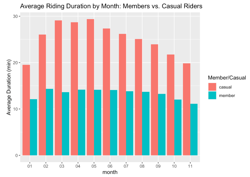
bikeshare2021_cleaned_v2 %>% group_by(month,member_casual) %>% 
  summarise(average_of_ride_time = mean(time_diff), .groups = 'drop') %>%
  ggplot(aes(x = month, y = average_of_ride_time, fill = member_casual)) +
  geom_col(position = 'dodge') +labs(x = "month", y = "Average Duration (min)", fill = "Member/Casual", title = "Average Riding Duration by Month: Members vs. Casual Riders")

Visual the Average Ride Time by Each Day for Memebrs vs Casuals Riders

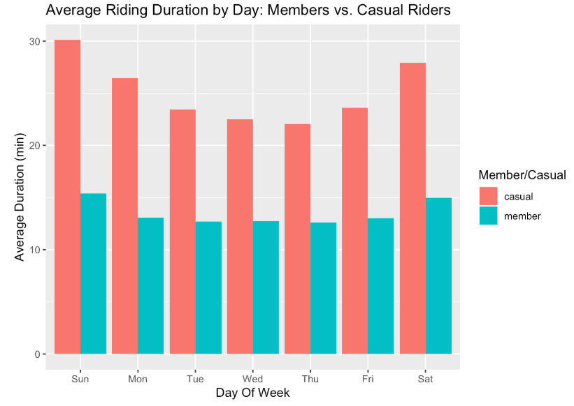
bikeshare2021_cleaned_v2 %>% group_by(dayof_week,member_casual) %>% 
  summarise(average_of_ride_time = mean(time_diff), .groups = 'drop') %>%
  ggplot(aes(x = dayof_week, y = average_of_ride_time, fill = member_casual)) +
  geom_col(position = 'dodge') + labs(x = "Day Of Week", y = "Average Duration (min)", fill = "Member/Casual", title = "Average Riding Duration by Day: Members vs. Casual Riders")
  

Visual the Average Number of Rides by Month: Member vs. Casual Riders

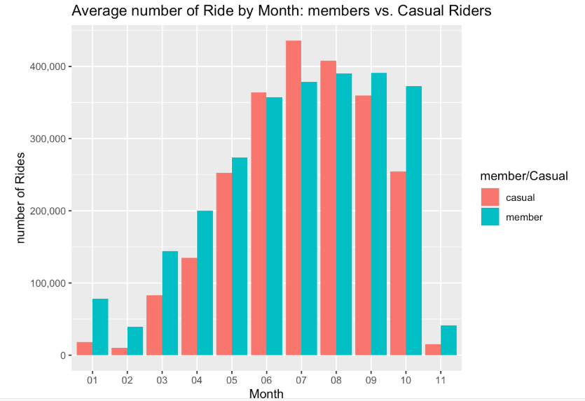
bikeshare2021_cleaned_v2 %>% 
  group_by(month, member_casual) %>% 
  summarise(number_of_rides = n(), .groups = 'drop') %>% 
  ggplot(aes(x= month, y = number_of_rides, fill = member_casual)) + geom_col(position = 'dodge') + scale_y_continuous(labels = scales::comma) + labs(x = "Month", y = "number of Rides", fill = "member/Casual", title = "Average number of Ride by Month: members vs. Casual Riders")

Visual the Average Number of Rides by Day: Members vs. Casual Riders

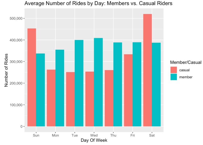
bikeshare2021_cleaned_v2 %>% group_by(dayof_week,member_casual) %>% 
  summarise(number_of_ride = n(), .groups = 'drop') %>%
  ggplot(aes(x = dayof_week, y = number_of_ride, fill = member_casual)) +
  geom_col(position = 'dodge')+scale_y_continuous(labels = scales::comma) +labs(x = "Day Of Week", y = "Number of Rides", fill = "Member/Casual", title = "Average Number of Rides by Day: Members vs. Casual Riders")

Visual for Number of Rides Grouped by Day: Rider Type

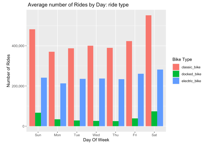
bikeshare2021_cleaned_v2 %>% group_by(dayof_week ,rideable_type) %>% 
  summarise(number_of_ride = n(), .groups = 'drop') %>%
  ggplot(aes(x = dayof_week, y = number_of_ride, fill = rideable_type)) +
  geom_col(position = 'dodge') + scale_y_continuous(labels = scales::comma) + labs(x= "Day Of Week", y = "Number of Rides", fill = "Bike Type", title = " Average number of Rides by Day: ride type" )

Visualfor Top 10 Used Start Stations

#replacing empty rows with NA
bikeshare2021_cleaned_v2[bikeshare2021_cleaned_v2 == ""] <- NA

#removing NA value 
bikeshare2021_cleaned_v3 <- na.omit(bikeshare2021_cleaned_v2)
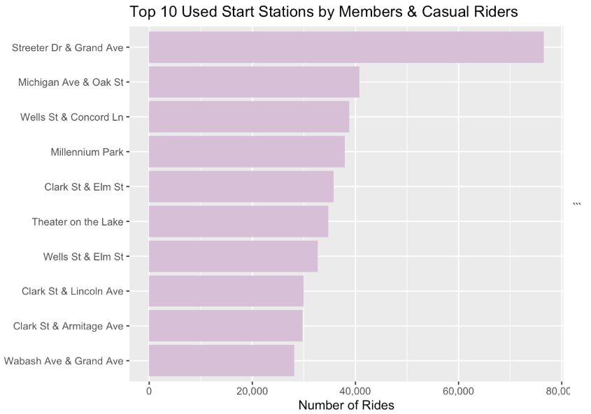
#get the top 10 popular start station for member and causal
top_10_start_staction_name <- bikeshare2021_cleaned_v3 %>% group_by(start_station_name) %>% summarise(station_count = n()) %>% arrange(desc(station_count)) %>% head(n = 10)

ggplot(data = top_10_start_staction_name)+ geom_col(aes(x = reorder(start_station_name, station_count), y = station_count), fill= "thistle") + coord_flip() + labs(title = "Top 10 Used Start Stations by Members & Casual Riders", y = "Number of Rides", x = "") + scale_y_continuous(labels = scales::comma)
  
  
 

Takeaways:

After performing the collection, transofrmation, cleaning, organization and analysis of the given 11 datasets, I have enought factual evidence to suggest anwsers to the business-related questions were asked.

I can infer that causal riders are mote likely to use their bike for a longer diration of time. Casual riders also preferred to ride in the weekened. fall and winter months is when user traffic drops for both types

To help convert Causal riders into buying annual membershipts, we have to refer the analysis provided above and keep in them in our mind. The recommendations I would provide to help solve this business-related scenario is shown below

Top Recommendations Marketing Strategist:

• Advertising annual memberships prices more in the top 10 most popular stations
• Provide a discount on annual membershipts purchase in winter and fall ( the lowest traffic months)
• advertise on social media during the peak months (mostly summer) - since that is when most people have a thought about riding bikes
• Condider provide free ride minutes for new member riders.

header | header | header data | data | data