For this project we'll be taking a look at housing sale data from the King's County Sales dataset, which can be found in kc_house_data.csv. Each record represents a house sale in the Seattle area for the year 2021-2022. Our Client, a real estate agency, specializes in the elusive mid-range home, and is looking for neighborhoods to target to increase their inventory. Our client would like to target the incorporated areas of Kings County, which as a whole covers roughly 10% of Washington state, and so we'll reduce the size of our dataset to reflect that change. We'll also keep our eye out for any features that might radically boost home price, such as waterfront properties, or homes adjacent to parks or greenways to provide a list of features or locations associated with inflated pricing- in other words, a "what to avoid".
Our first steps were to import our libraries and clean our data. This included dropping a small number of NaN entries, identifying invalid entries, and starting the process of identifying and eliminating outliers. Of the 30155 records included in the original kc_house dataset we used 21059, eliminating 819 erroneous files. In its raw form the 30,155 homes in the kc dataset have a mean price of 1,108,536 dollars, a mean size of 2112 sqft, and 3.4 bedrooms.
.
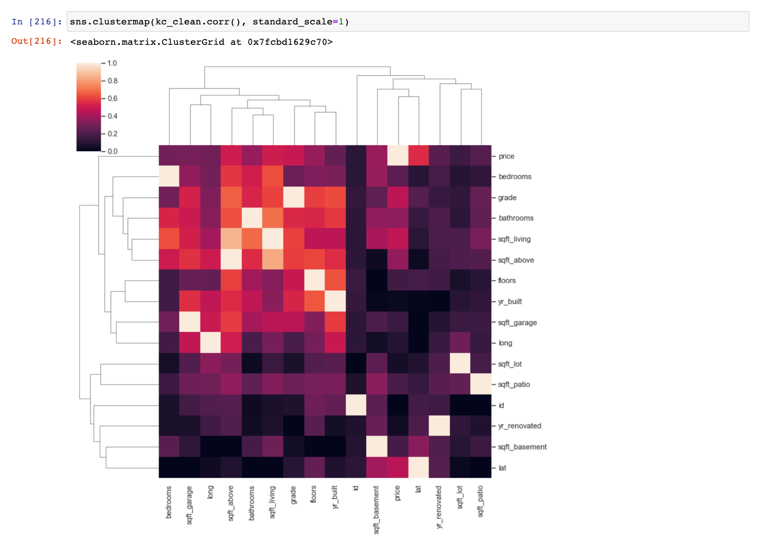
With possible predictors from the original columns, and our engineered column of 'zip', there were over 26 possibilities to examine. Using our clients interests, and a variety of tools(correlation matrices, scatterplots and simple linear regression models) we were able to pare down our list to three target predictors that became clear frontrunners for inclusion in our final models: 'zip', 'grade', and 'sqft_living'.
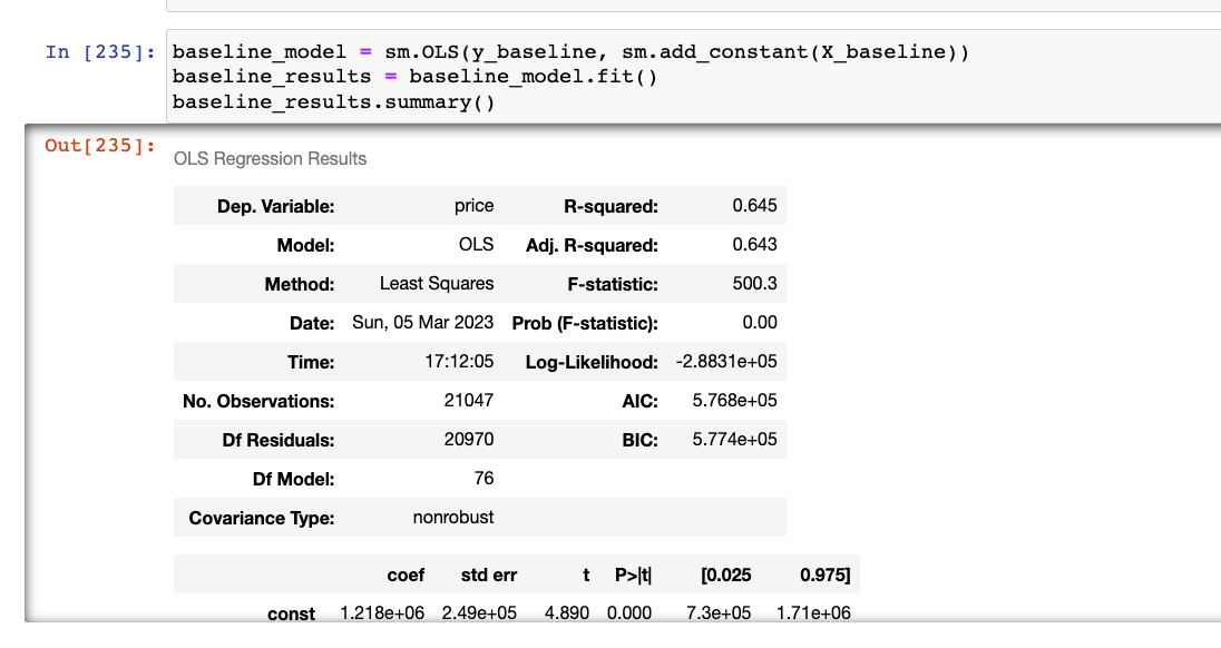
Using an OLS model we were able to identify the impact of both a homes quality (grade) on the mean price, as well as prove that certain amenities are just too pricey to justify for a midrange home, such as waterfront access, homes in above average condition. Our centered data resulted in a model r-squared of 64%, an intercept (in this case, average price) of 884,000.
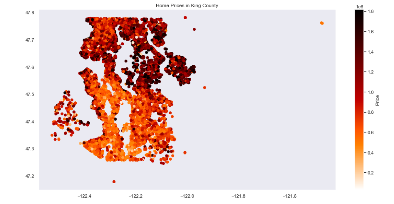
Using our final model we identified which neighborhoods we would be able to locate housing in two distinct areas that would be in the lowest mean price by zipcode. South of SeaTac: 98023: Federal Way, 98092: Auburn, 98422:Tacoma, 98030: Kent and east of Mercer Island in the neighborhoods of Issaquah and Bellevue.
We can also see that we'll want to look for houses that are in low to average grade, as we see prices jumping over the median once we've crossed the average grade threshold. Additionally, while we'll want to avoid waterfront homes because of the significant jump in price (about a 100,00 dollars), our real estate agent might want to target homes that are located near greenbelts or parks, which have a significantly lower jump in price- around 8,000.
Our model had a large MAE (about 160,00) even for home prices, and the plot of our residuals demonstrated imperfect distribution, challenging the accuracy of our model.
Affordable housing is a challenge to find in the best of times, and often neighborhoods with lower housing prices are located nearby inherent health dangers like freeways or large industrial areas, or lack the kinds of amenities that enhance quality of life, like greenspaces and grocery stores. Our next steps would be to overlay a map of such amenities or dangers over the neighborhoods we've identified as being our most affordable, to analyze the additional benefits and risks of those neighborhoods and to allow our client to have a fuller understanding of its benefits or disadvantages.