Mechanical Design Workflow

This repository serves two purposes:

1. A quick visual map of the Python packages available to designers: Python for the Design Desk, below. There's nothing to install; just scroll down and read.
2. A starting point for any AI coding agent: download the repository, start an agent in it, give it a problem, and let it not only solve the problem, but also write a detailed and educational report. Section 3 shows how, step by step.

Neither needs you to write code. For the second, the agent writes and runs the Python. Your job is to state the problem and review its answer.

This is a proof of concept for one idea: an analysis shouldn't quietly inherit a bad assumption. It ties together a structured way to make design decisions, a written record of every assumption, and analysis in Python, with a clear path from framing the problem to sign-off. It holds a design checklist, a design-record template, and a worked Python FEA example checked against the textbook answer, the closed-form solution and a second FE package.

There is one worked example so far. The rest of this page maps Python packages to design jobs, compares free alternatives to MATLAB and Simulink, and lists gotchas: traps that run without an error and still give a wrong answer. A separate file, Python for Hydraulics, surveys the same ground for pipe networks, rivers, stormwater, groundwater and fluid power.

Start here

You want to	Do this	You need
Find the right Python package for a job	Read the map. It's organized by job, with a picture and a short example for most packages	Nothing: it's on this page
See what a finished analysis looks like	Open the worked example's PDF sample, a 13-page printed calculation	Nothing: GitHub shows the PDF in your browser
Solve your own problem	Follow section 3: download this repository, open it in an AI coding agent, and describe the problem	An AI coding agent (most need a paid subscription) and a computer you can install Python on
Run the notebooks yourself	Follow Setup, then open a notebook in Jupyter or VS Code	Python 3.11

Words you'll meet

• Repository (or repo): a project's files and their history, hosted on GitHub. This page is the front of this one. Download ZIP gives you the current files as an ordinary folder, without the history.
• AI coding agent: a language model run by a tool, the harness, that lets it read and write files in a folder on your computer and run commands there, with your approval. Claude Code, OpenAI Codex, Cursor and GitHub Copilot's agent mode are harnesses.
• Notebook (.ipynb): a Jupyter document that mixes explanation, Python code and its saved output: equations, plots and tables. GitHub renders one as a page, so you can follow it without reading the code.
• Virtual environment (venv): a self-contained Python installation in its own folder, holding the exact package versions pinned in requirements.txt, so they don't clash with anything else on your computer. The agent can create it for you.
• The checklist and the traveller: the method this repository follows, and the record it fills in for each part. Section 1 describes both.
• PASS/FAIL checks: the table at the end of every notebook that compares each result with an independent one. If any check fails, the last cell raises an exception, so a failure can't pass unnoticed.

1. The design and analysis framework

There are two documents: reference material, and the working record for a part.

• The checklist is a decision tree for the common 80% of mechanical design: static loads, linear-elastic response, and standard strength and deflection limits. It doesn't try to cover everything. A triage gate screens for nine specialized regimes, including fatigue, fracture and creep, and routes any that apply out for separate analysis. The key piece is the Assumption Ledger, where every idealization the math depends on, such as Euler-Bernoulli vs. Timoshenko or linear elasticity, gets written down.
• The traveller is a blank design-record template, copied for each part. It keeps the checklist's checkboxes, decision trail, Assumption Ledger audit and sign-off blocks, without the explanations. It is built for review: it makes you state the governing failure mode and the margin of safety.

2. The worked example

_{Problem after R. C. Hibbeler, Mechanics of Materials, 8th ed., Example 1.1. Figure drawn for this repository.}

Cantilever_Beam_Analysis_Triangular_Load.ipynb solves this beam four ways and checks each against the others:

• The closed form, derived in SymPy from the load function and checked symbolically against the textbook tables. The problem statement and theory are written in LaTeX, and each equation is cited to Shigley's Mechanical Engineering Design or Hibbeler's Mechanics of Materials by number and printed page.
• A hand-calculation record in handcalcs and pint, which shows every substitution with its units. It reproduces Hibbeler's own solution of Example 1.1.
• PlaneSections, which uses PyNiteFEA as its solver, with the linear load applied exactly. One four-panel figure shows the shear, moment, deflection and slope against the closed form.
• anaStruct, a second FE package built separately, as the independent check.

Every number lands on the textbook answer: wall reaction 1215 N, wall moment 3645 N·m (hogging), and at C a shear of 540 N and a moment of 1080 N·m (hogging). The tip deflection is 0.656 mm. The notebook ends with 29 PASS/FAIL checks, and its last cell raises if any fails. To read it as a printed calculation, open the 11 × 17 in PDF sample (13 pages, typeset with LaTeX).

It also writes the Assumption Ledger out, with a link to each checklist node. Euler-Bernoulli beam theory, linear elasticity and small deflection all hold by wide margins. Self-weight doesn't: the textbook neglects it, and the solid steel section this notebook assumes would weigh 17 times the load it carries. The notebook says so and shows what superposing it would change.

Some packages can't apply a linearly varying load, so the taper has to be split into constant-load strips. A convergence study shows what that costs: doubling the number of strips quarters the error in the root moment, and 72 strips still leave it 0.0096% off.

3. Solve your own problem with an AI coding agent

The agent writes the Python, runs it and writes it up. AGENTS.md holds the rules it follows here, and CLAUDE.md imports the same file for Claude Code. The rules: frame the problem with the checklist before computing, route out any specialized regime, check every result independently, audit the Assumption Ledger against the answer, and leave sign-off to the engineer.

What you need

• An AI coding agent that can work on a local folder, such as Claude Code (in the Claude desktop app or a terminal), OpenAI Codex, Cursor, or GitHub Copilot's agent mode in VS Code. Most need a paid subscription. A chat assistant in a web page can explain these files, but it can't execute the notebooks.
• Python on your computer. If it isn't installed, the agent will tell you and walk you through installing it. The pinned packages are tested on Python 3.11.
• No GitHub account. The repository is public, so anyone can download it.

Step by step

1. Download this repository. At the top of this repository's page, click the green Code button, then Download ZIP. (If you use git, git clone https://github.com/thomastron/Mechanical-Engineering-Python.git instead, and skip step 2.)
2. Unzip it. On Windows, right-click the zip file and choose Extract All; on a Mac, double-click it. Put the folder somewhere you'll find it again, such as Documents.
3. Open the folder in your agent. Start the agent with the unzipped folder as its working directory. Claude Code loads CLAUDE.md from there automatically; Codex, Cursor and Copilot read AGENTS.md.
4. Ask it to set up. For example: "Create the virtual environment from requirements.txt, then execute the worked example and confirm all its checks pass." The first install takes a few minutes. The agent asks before running each command: read what it's about to run, and approve only what you understand.
5. Give it a problem. Type it, paste it, or attach a photo of a textbook page or a sketch, and say what you want back. For example:
   • "Solve this problem from Hibbeler's Mechanics of Materials two independent ways, in a new notebook."
   • "A steel shelf bracket holds 50 kg, 300 mm from the wall. Is a 6 mm plate thick enough? Use the checklist and fill in a traveller."
   • "Explain every step as if I'm a first-year student."
6. Read what it made. Expect these in the folder:
   • a new notebook with the problem, the theory, each step, plots and the PASS/FAIL table;
   • a filled-in copy of the traveller, with every assumption written down and anything it routed out;
   • a report to read or print, if you ask for one. nbconvert exports an HTML copy that opens in any browser, with nothing more to install. A PDF like the sample goes through LaTeX (pandoc plus a TeX distribution), which the agent can help you install.
7. Review it. Read the Assumption Ledger and the governing number first. Ask why about anything you don't follow, and ask for another method if a result looks wrong. The agent never signs anything off: that stays with the engineer.

Things to know

• You can't break anything here. A download or clone is your own copy. Nothing you do in it reaches this repository.
• The agent runs commands with your user permissions. Most harnesses ask before each one, and some can sandbox them. Work in the downloaded folder, not one that holds files you care about.
• The model can be wrong. That's why every result is checked a second way and every assumption is written down. Treat its output as a calculation to review, not an answer to trust.
• The method covers static, linear-elastic design. Fatigue, fracture, creep, contact, impact and the other specialized regimes are flagged at the triage gate and routed out, not quietly solved with the wrong method. The agent should tell you when that happens.

4. Standard workflow

To work a problem yourself, or to follow what the agent is doing:

1. Frame and model. Use the checklist to set the problem's criticality, the load paths, and the right idealizations.
2. Compute. Build a tractable model in a Jupyter notebook and extract the internal resultants.
3. Document. Record the decisions, bounds and limits in a fresh copy of the traveller.
4. Audit. Run the final numbers back through the traveller's Assumption Ledger. Check that the computed stresses and deflections don't break the linear-elastic or small-deflection assumptions you started with.

5. Setup

This is what step 4 of section 3 asks the agent to do, for anyone who'd rather do it by hand. Tested on Python 3.11.

python -m venv .venv

Activate it (.venv\Scripts\activate on Windows, source .venv/bin/activate on macOS and Linux), then:

pip install -r requirements.txt

requirements.txt pins every Python package in the map below. A few entries need more than pip:

• Not pip packages. GXBeam is a Julia package. FEniCSx has no pip wheels (see its section for conda and Docker). GNU Octave and OpenModelica are standalone programs: oct2py needs Octave on the PATH (Debian/Ubuntu: sudo apt install octave), and OMPython needs OpenModelica. CalculiX is a standalone solver: PrePoMax bundles it on Windows, and Debian/Ubuntu package it (sudo apt install calculix-ccx). See its section for how the notebook finds it.
• System libraries on Linux. openseespy needs BLAS and LAPACK, and Gmsh, the mesher behind EasyFEA and CALFEM, needs libGLU and libXft (Debian/Ubuntu: sudo apt install libblas3 liblapack3 libglu1-mesa libxft2).
• Compared, not pinned. SimuPy, because its last release doesn't import on NumPy 2.

Run a notebook headless to check that it still passes. The second line checks the whole environment:

MPLBACKEND=Agg jupyter nbconvert --to notebook --execute Cantilever_Beam_Analysis_Triangular_Load.ipynb --inplace
MPLBACKEND=Agg jupyter nbconvert --to notebook --execute Design_Desk_Smoke_Test.ipynb --inplace

Design_Desk_Smoke_Test.ipynb has 138 checks in its committed run. Every pinned analysis package solves a problem with a known answer (nine of them solve the same cantilever), and every installed version is compared with its pin. If a check fails, the last cell raises and the command exits non-zero. Checks that need Octave, OpenModelica or CalculiX report as skipped, not passed, when those programs aren't installed.

CalculiX_Validation_Checks.ipynb needs CalculiX itself. Run it without MPLBACKEND=Agg: under Agg, plt.show() has nothing to draw, so the saved notebook loses its plots.

---

Python for the Design Desk

Organized by the job, not the package. Each name links to its section.

Hydraulics has its own map. Python for Hydraulics covers water distribution networks (EPANET, through wntr and epyt), pipe, valve and pump sizing with fluids, open channels and floodplains (HEC-RAS, anuga), stormwater and sewers (pyswmm), groundwater (flopy), CFD, and fluid power. It is a survey, not a checked set like this one: none of its packages are pinned in requirements.txt, and none have been run here yet.

The job	Reach for
Writing up and checking a calculation
Document a calculation so a reviewer can audit it	handcalcs
Keep units straight across kpsi and SI	pint (forallpeople if SI-only)
Carry tolerance and scatter through a formula	uncertainties, scipy.stats
Notebook → PDF, or any HTML → PDF / PNG	nbconvert, playwright
Beams, frames and sections
Quick beam diagrams	planesections (numeric), symbeam (symbolic)
2D frame and truss analysis	anastruct, Pynite
Torsion in a shaft (diagram, internal T)	Pynite ('MX' loads, torque_array)
Cross-section properties, arbitrary shapes	sectionproperties
Finite elements
Assemble the global stiffness matrix yourself	calfem-python (imports as calfem)
Nonlinear and seismic structural analysis	openseespy
2D/3D solid FEA without writing the weak form	EasyFEA
Weak-form FEA in pure Python, installed with pip	scikit-fem (imports as skfem)
Solids, beams, buckling and contact from an established solver	CalculiX, a standalone program run from Python
Weak-form FEA at scale, compiled and parallel	FEniCSx (dolfinx)
Full-wave electromagnetic FEA (RF, S-parameters)	rapidfem
Large-deflection / geometrically exact beams	GXBeam.jl
Symbolic math and mechanisms
Symbolic derivation, algebra, calculus	sympy
Beam by singularity functions, symbolically, hinges included	sympy.physics.continuum_mechanics.beam
Multibody dynamics: Kane's method, Lagrange	sympy.physics.mechanics (PyDy's core)
Linkage, cam and spur-gear kinematics	mechanism
Numerics
Root-finding, curve fits, ODEs, eigenvalues	scipy
Fatigue cycle counting from a load history	wetb.fatigue_tools
MATLAB and Simulink alternatives
Run existing MATLAB .m code, or check a port	GNU Octave, via oct2py
Transfer functions, Bode, root locus, margins	control (python-control)
Simulink-style block-diagram simulation	pathsim
Simscape-style physical (acausal) models	OpenModelica, driven by OMPython
Run an exported model (an FMU) from Python	fmpy
Put an FMU inside a block diagram	pathsim-fmi

Writing up and checking a calculation

handcalcs

repo

Use for: Writing a calculation in Python and getting it back as rendered, step-by-step LaTeX: a hand calculation a reviewer can audit. Use pint for the units. The first five gotchas are about this pairing. The worked example uses its @handcalc decorator, which keeps the record's variables inside a function, so names like L don't overwrite the notebook's own.

_{Image: handcalcs README, © Connor Ferster, Apache-2.0.}

uncertainties

docs · repo

Use for: Carrying tolerances, material scatter and measurement error through a formula without deriving the propagation by hand. Write each input as a value ± its standard deviation. The result carries its own, and error_components() tells you which input it came from.

The shaft sized in the SciPy examples has n = 2.0. Give its inputs some scatter:

from math import pi
from uncertainties import ufloat

d  = ufloat(1.697, 0.002, "d")     # shaft diameter [in], 1σ
M  = ufloat(12_000, 1_200, "M")    # bending moment [lbf·in], 1σ
Sy = ufloat(50_000, 2_500, "Sy")   # yield strength [psi], 1σ

n = Sy * pi * d**3 / (32 * M)      # factor of safety against yield
print(n)                           # 2.00+/-0.22
for var, err in n.error_components().items():
    print(var.tag, round(err, 3))  # M 0.2, d 0.007, Sy 0.1

The load scatter dominates. Tightening the diameter tolerance buys almost nothing; pinning down the load buys the most.

Checked: 3.2.3. The propagation is first order, so it assumes each input's scatter is small. A Monte Carlo run of the same inputs (2 × 10⁶ samples) gives n = 2.02 ± 0.23. The linear estimate is 4% low on the scatter and misses a 1% shift in the mean, because n goes as 1/M. For wide scatter, or a probability of failure, sample with scipy.stats instead.

nbconvert

docs

Use for: Turning a finished notebook into a PDF, HTML or LaTeX record, with the outputs in place. Add --no-input for a clean calc report: outputs and markdown only.

Route to PDF	Command	Verdict
LaTeX (needs TeX, such as MiKTeX or TeX Live, plus Pandoc)	jupyter nbconvert --to pdf "X.ipynb"	Use this to print. Wraps long lines, so nothing is lost, and typesets the math
Browser, via Playwright	jupyter nbconvert --to webpdf "X.ipynb"	Looks like the notebook on screen, but cuts off anything wider than the page. On Windows, see the gotchas

Bigger paper. The LaTeX template sets the page size in one block, margins, and defaults to letter. Override just that block for Tabloid (11 × 17 in): save this as tabloid.tex.j2 and add --template-file tabloid.tex.j2.

((*- extends 'index.tex.j2' -*))
((* block margins *))
\geometry{verbose,paperwidth=11in,paperheight=17in,tmargin=1in,bmargin=1in,lmargin=1in,rmargin=1in}
((* endblock margins *))

In one test, a notebook went from 22 letter pages to 13 on Tabloid. Swapping the sizes gives Ledger (17 × 11 in), which saves no pages, since its usable height is letter's 9 in, but long lines and wide tables stop wrapping.

Playwright

docs

Use for: HTML → PDF or PNG: a styled pandas table, an HTML calc sheet, or a whole notebook through nbconvert --to webpdf. Playwright drives a real browser from Python. After pip install playwright, run python -m playwright install chromium, which downloads a matched browser build (several hundred MB, outside the project; re-run it after upgrading). To learn the API, python -m playwright codegen --target=python https://example.com writes the Python as you click.

Beams, frames and sections

PlaneSections

repo

Use for: Quick 1D beam analysis and clean shear and moment diagrams for ordinary load cases. The worked example uses it.

_{Images: planesections README, © cslotboom, Apache-2.0.}

SymBeam

repo

Use for: Exact shear, moment and deflection of a beam as algebra, not numbers. It was written for teaching, and it shows each piecewise expression.

_{Image: SymBeam README, © 2020 António Carneiro, MIT License.}

anaStruct

docs

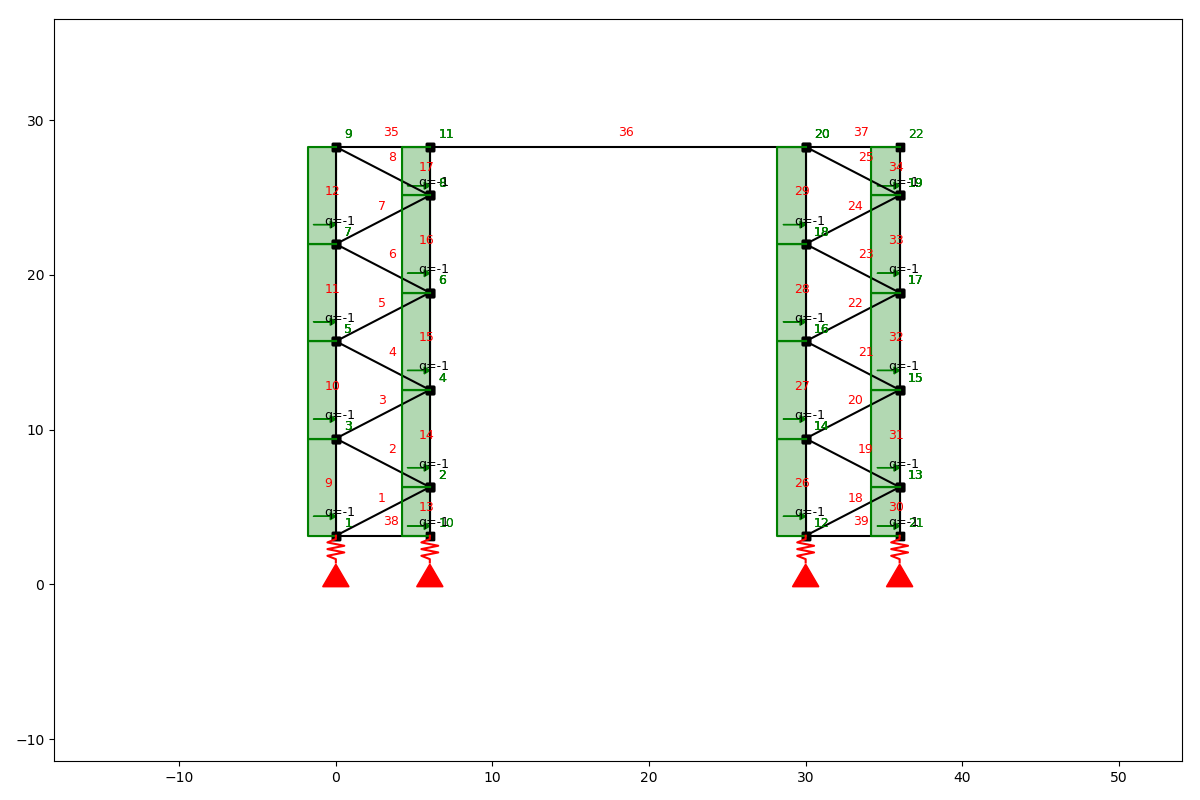
Use for: Quick 2D analysis of frames and trusses: bending moment, shear and axial force diagrams. It handles internal hinges natively, and its forces are exact there, but its hinged deflections are not. Check any deflection near a hinge independently. The worked example uses it as its independent check. Its signs differ from the textbook's (see Gotchas).

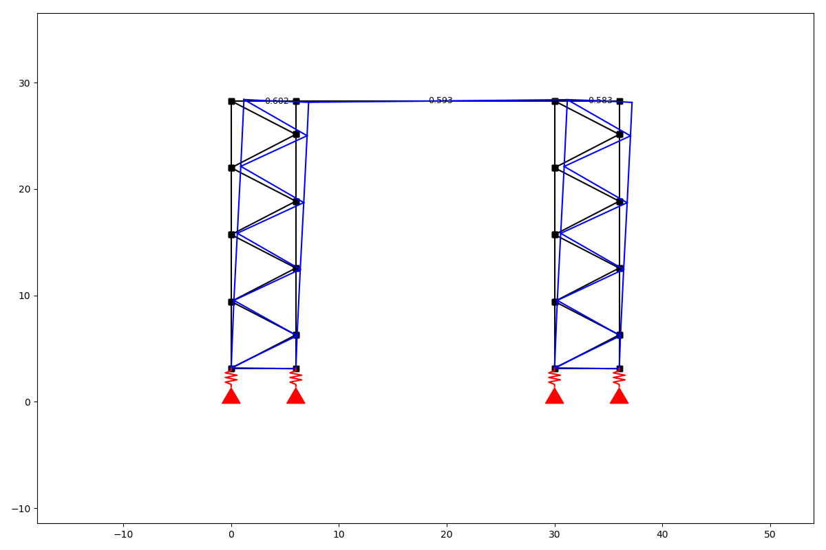_{Images: anaStruct documentation, © Ritchie Vink and anaStruct contributors, LGPL-3.0.}

Pynite

docs · repo

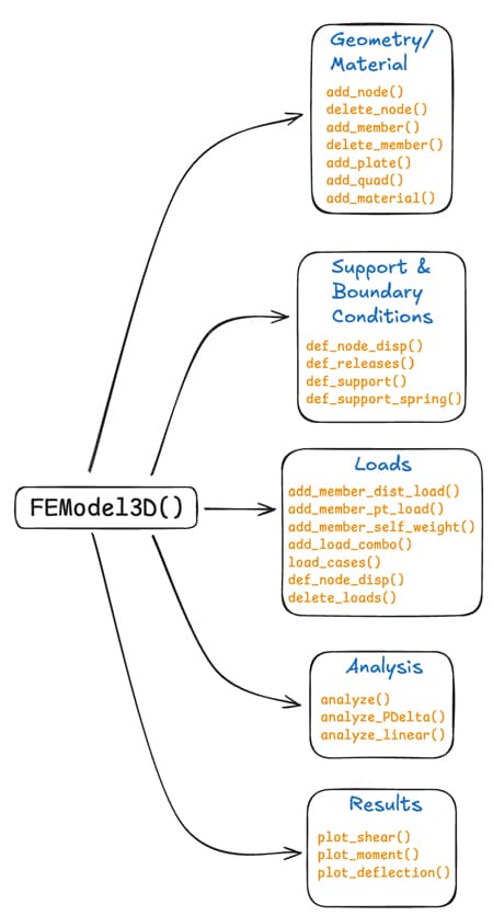
Use for: 3D frames, trusses and plates: member shear, moment, torsion and deflection, with P-Δ when the axial load matters.

_{Left: from A Pynite Crash Course by Seán Carroll, © EngineeringSkills.com. Right: animation from Connor Ferster's LinkedIn post, © Connor Ferster.}

sectionproperties

docs

Use for: Properties of any cross-section you can draw: area, second moments, torsion constant and shear center, plus the stress over the section. Custom extrusions and built-up shapes are the point.

_{Images: sectionproperties documentation, © Robbie van Leeuwen, MIT License.}

Finite elements

The FE packages in this map cover very different ground. Roughly from least setup to most:

Tool	What it models	Physics	You supply	Install on Windows
PlaneSections	1D beams	Linear statics, SFD/BMD	Supports and loads	pip
anastruct	2D frames and trusses	Statics, mainly linear	Nodes, elements, loads	pip
Pynite	3D frames, plates	Linear and P-Δ statics	Nodes, members, loads	pip
sectionproperties	2D cross-sections	Section properties, stress over the section	Section geometry	pip
CALFEM	Springs, bars, 1D–3D beams, plane and 3D solids, plates, heat flow	Linear statics, vibration modes, heat and potential flow	Element matrices, the DOF numbering, the assembly loop	pip
OpenSeesPy	Frames and continua	Nonlinear static and dynamic, seismic	Elements, materials, analysis steps	pip
EasyFEA	2D/3D solids, meshed with Gmsh	Elasticity, hyperelasticity, plasticity, contact, phase-field fracture, thermal, beams	Geometry, model, boundary conditions	pip
scikit-fem	1D/2D/3D; simple meshes built in, others imported	Any PDE you can write as a weak form; ships elasticity, plate (Morley, Argyris) and beam (Hermite) elements	The weak form, the mesh, the boundary conditions	pip
CalculiX	1D beams, 2D and 3D solids, shells; meshed with Gmsh or PrePoMax	Linear and nonlinear statics, buckling, natural frequencies, contact, plasticity, heat transfer	An Abaqus-style .inp input deck	standalone program (bundled with PrePoMax)
FEniCSx	1D/2D/3D, any mesh	Any PDE you can write as a weak form	The variational formulation	conda, Docker or WSL
RapidFEM	3D, built-in mesher	Full-wave Maxwell (RF and microwave)	Geometry, materials, ports	pip

CALFEM

docs · manual · repo

Use for: Finite element analysis you can follow line by line. Every other FE tool here is a black box, and the stiffness matrix never leaves the solver. CALFEM hands you the element matrices (springs, bars, 1D to 3D beams, plane and brick solids, plates, heat flow) and makes each step of the direct stiffness method a function call: beam2e builds an element matrix, assem adds it into the global K, solveq applies the supports and solves, and beam2s recovers the section forces. You can print K, check its symmetry and eigenvalues, and compare any entry with a hand calculation.

Where it fits: Learning FE, and checking a black-box frame result from anastruct or Pynite step by step. It is not for production models: apart from a few second-order bar and beam elements it is linear elastic, with no plasticity or contact, and you write the assembly loop every time. The name stands for Computer Aided Learning of the Finite Element Method; Lund University has developed it since the late 1970s, and this is the Python port of the MATLAB original. MIT License.

Checked: 3.6.16. The snippet below gives a tip deflection of 25.600 mm, matching PL³/3EI to 4 × 10⁻¹⁶, wall reactions of 1000 N and 2000 N·m, and a symmetric K with exactly three zero eigenvalues.

_{Figure: drawn for this README from the K that the snippet below assembles. Each 2D beam element has two nodes with three DOFs each (u, v, θ), so its matrix is 6 × 6. Assembly adds it into the rows and columns of its DOFs, so where two elements share a node their entries add, the way springs in parallel add. Every empty cell is an exact zero.}

What K tells you.

• It must be symmetric, by Maxwell–Betti reciprocity. An asymmetric K is an assembly error.
• It is singular until the structure is supported. Rigid-body motions take no force, so the unsupported cantilever has three zero eigenvalues: sliding along x, sliding along y, and rotating. A zero eigenvalue that survives the supports is a mechanism, such as a missing support or a hinge in the wrong place. That is what a solver's "singular matrix" error means.
• Its condition number bounds how much round-off the solve can amplify. Stiff and flexible load paths in one model raise it; in a slender beam, EA/L is far larger than 12EI/L³. Here it is 6.7 × 10⁴, harmless in double precision.

solveq(K, f, bc) returns the reactions as well as the displacements. Check them against statics: here they must equal P and PL. The gotchas show a support error that passes the deflection check and fails this one.

The snippet: the cantilever in the figure, 2 m of 50 × 50 mm steel with a 1 kN tip load

import numpy as np
import calfem.core as cfc

E, A, I = 200e9, 0.05**2, 0.05**4 / 12  # steel, 50 x 50 mm [Pa, m^2, m^4]
P = 1000.0                              # tip load [N]

# Three DOFs per node: u (axial), v (transverse), θ (rotation), numbered from 1
edof = np.array([[1, 2, 3, 4, 5, 6],    # element 1: node 1 to node 2
                 [4, 5, 6, 7, 8, 9]])   # element 2: node 2 to node 3
ex = [[0.0, 1.0], [1.0, 2.0]]           # x of each element's two ends [m]

K = np.zeros((9, 9))
for dofs, x in zip(edof, ex):
    Ke = cfc.beam2e(x, [0.0, 0.0], [E, A, I])  # this element's 6 x 6 matrix
    cfc.assem(dofs, K, Ke)                      # add it into the global K

f = np.zeros((9, 1))
f[7] = -P                       # DOF 8 (v at node 3) is NumPy index 7
bc = np.array([1, 2, 3])        # clamped at the wall: u, v, θ of node 1
a, r = cfc.solveq(K, f, bc)     # displacements a, reactions r

print(np.allclose(K, K.T))              # True: K is symmetric
print(np.linalg.eigvalsh(K)[:3])        # three ~0 eigenvalues: rigid-body modes
print(-a[7, 0] * 1e3)                   # 25.6 mm, = PL³/3EI
print(r[1, 0], r[2, 0])                 # 1000 N and 2000 N·m at the wall

Two elements give the exact answer here, not a converged one: beam2e uses cubic shape functions, and an Euler–Bernoulli beam loaded only at its nodes deflects as a cubic between them. Agreement with PL³/3EI shows the assembly is right. It is not a mesh study.

OpenSeesPy

docs

Use for: Nonlinear structural and geotechnical FEA, static or dynamic: seismic response, plastic hinges, and advanced material models.

_{Images: OpenSeesPy documentation, © Minjie Zhu. OpenSeesPy license: free for research, education and internal use; commercial redistribution needs a license.}

EasyFEA

docs

Use for: 2D and 3D solid-mechanics FEA without writing the weak form: elasticity, hyperelasticity, plasticity, contact, phase-field fracture, thermal, and beams. You mesh with Gmsh through its geometry classes, pick a model, apply boundary conditions and solve.

Where it fits: The step up from frame solvers to real 2D and 3D stress fields, limited to the physics it ships. The project calls itself emerging. GPL-3.0, from Université Gustave Eiffel.

Checked: 7.0.0 (pip install "EasyFEA[viz]", which pulls in Gmsh and PyVista). A 2 m steel cantilever, 50 × 50 mm, with a 1 kN tip load deflected 25.600 mm, matching PL³/3EI to 2 × 10⁻¹¹.

_{Images: EasyFEA documentation gallery, © Université Gustave Eiffel and INRIA (Matthieu Noel), GPL-3.0.}

scikit-fem

docs · gallery · repo

Use for: Weak-form FEA in plain Python. You write the bilinear and linear forms as short functions, and scikit-fem assembles them into SciPy sparse matrices. The elements run from high-order Lagrange through Hermite beams and Morley and Argyris plates to Nédélec elements. It is pure Python on NumPy and SciPy, so pip install scikit-fem works wherever Python does. BSD-3-Clause, described in a 2020 JOSS paper.

Where it fits: FEniCSx's job without the conda or Docker install, for models a laptop can solve directly. It shares no element or assembly code with EasyFEA, so it is a good independent check on an EasyFEA stress result. It is an assembler, not an analysis package:

• Meshes: simple ones are built in. Anything else comes from Gmsh, through meshio (not in requirements.txt), or as arrays.
• Solvers: SciPy's sparse direct solve, which limits 3D models. The project's own benchmark (linear tetrahedra, on a laptop) takes 11 s for 33 000 DOFs and 63 s for 64 000.
• Nonlinear problems: you write the Newton loop, or use the optional JAX-based skfem.autodiff.
• Stresses: yours to compute from the displacement gradient.

Checked: 12.0.2.

• The cantilever from the CALFEM and EasyFEA sections, with two cubic Hermite elements and the weak form ∫ EI w″v″ dx: 25.600 mm, matching PL³/3EI to 4 × 10⁻¹⁶, and wall reactions of 1000 N and 2000 N·m.
• A thick-walled cylinder against Lamé's closed form (100 mm bore, 200 mm outside diameter, steel, 100 MPa, plane strain, quadratic triangles): bore displacement 47.65 μm against 47.67 μm (3.8 × 10⁻⁴), and peak hoop stress on the bore 166.90 MPa against 166.67 MPa (0.14%). The reaction across the symmetry plane equals p·rᵢ to round-off. That is equilibrium, so it holds on any mesh: it catches sign and boundary-condition errors, not discretization error.
• A mesh study (the figure). The hoop-stress error falls roughly as h², from 3.8% to 0.12%. Straight element edges on the curved bore cap convergence at h², even for quadratic elements. Curved edges (MeshTri2) make the bore displacement 20 times more accurate on the finest mesh but leave the stress error almost unchanged, and the stress is the governing number.

_{Figure: drawn for this README from the snippet below, with the hoop stress evaluated from the displacement gradient on the bore facets.}

The snippet: the Lamé cylinder, a quarter section with symmetry planes

import numpy as np
from skfem import (MeshTri, Basis, FacetBasis, ElementTriP2, ElementVector,
                   LinearForm, condense, solve)
from skfem.helpers import dot
from skfem.models.elasticity import linear_elasticity, lame_parameters

E, nu = 200e9, 0.3                # steel [Pa, -]
ri, ro, p = 0.05, 0.10, 100e6     # bore and outside radius [m], internal pressure [Pa]

# Quarter of the cross-section: a 16 x 32 grid in (r, θ), mapped to (x, y)
m = MeshTri.init_tensor(np.linspace(ri, ro, 17), np.linspace(0, np.pi / 2, 33))
r, th = m.p
m = MeshTri(np.array([r * np.cos(th), r * np.sin(th)]), m.t).with_boundaries({
    "bore": lambda x: np.hypot(*x) < 1.001 * ri,  # facet midpoints sit just inside the arc
    "y0": lambda x: np.isclose(x[1], 0.0),        # symmetry plane: v = 0
    "x0": lambda x: np.isclose(x[0], 0.0),        # symmetry plane: u = 0
})
basis = Basis(m, ElementVector(ElementTriP2()))   # quadratic triangles
bore = FacetBasis(m, basis.elem, facets="bore")

# The weak form: ∫ σ(u) : ε(v) dΩ = ∫ t · v dΓ, with the traction t = −p n on the bore
K = linear_elasticity(*lame_parameters(E, nu)).assemble(basis)  # 3D λ, μ: plane strain
f = LinearForm(lambda v, w: dot(-p * w.n, v)).assemble(bore)
D = np.concatenate([basis.get_dofs("y0").all("u^2"), basis.get_dofs("x0").all("u^1")])
u = solve(*condense(K, f, D=D))

A = p * ri**2 / (ro**2 - ri**2)
node = np.flatnonzero(np.isclose(m.p[0], ri) & np.isclose(m.p[1], 0.0))[0]  # bore, on the x axis
print(u[basis.nodal_dofs[0, node]] * 1e6)                           # 47.65 μm
print((1 + nu) / E * A * ((1 - 2 * nu) * ri + ro**2 / ri) * 1e6)    # 47.67 μm, Lamé
print(-(K @ u - f)[basis.get_dofs("y0").all("u^2")].sum() / 1e6)    # 5.000 MN/m = p·ri

lame_parameters makes a 2D model plane strain, which is right for a long cylinder. A thin plate needs plane_stress, and mixing them up raises no error (see the gotchas).

From the project's gallery, all solid mechanics:

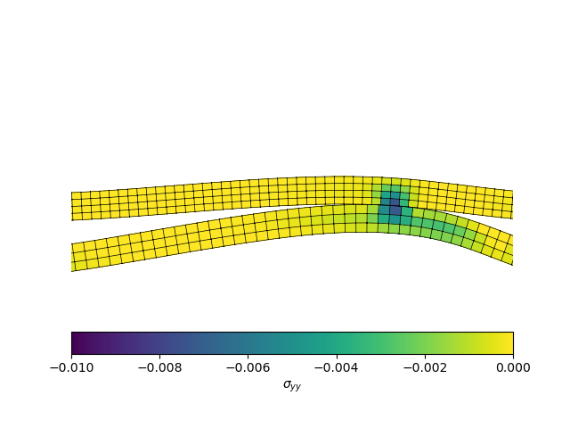Kirchhoff plate bending, Morley elements	Elastic vibration, fifth mode	Large-deformation contact (needs JAX)

_{Images: the scikit-fem gallery, © scikit-fem developers, BSD-3-Clause. Examples 2 and 3 were rendered for this README by running the gallery's own code, unchanged, with scikit-fem 12.0.2. Example 51 is the image from the project's repository.}

CalculiX

site · PrePoMax · notebook

Use for: A general-purpose FE solver with an Abaqus-style input deck: quadratic solid elements, beams and shells (which it expands internally into solids), linear buckling, natural frequencies, contact, plasticity and heat transfer. Python writes the .inp file as text, runs ccx with subprocess, and parses the text results, so there is no Python binding to install. CalculiX is GPL-2.0-or-later. PrePoMax, the free Windows GUI that bundles it, is GPL-3.0. The notebook calls the solver as a separate program and ships none of its code.

Where it fits: Reach for it when a model needs what scikit-fem and EasyFEA don't ship ready-made, such as linear buckling, contact, or beam and shell elements beside solids, all from one established solver. Meshing is separate. Gmsh builds the mesh, and two of the gotchas are in that hand-off. The deck is plain text, so a model can be diffed and reviewed like code.

Install: a standalone program, not a pip package. On Windows, unzip PrePoMax and keep its whole Solver folder together, because ccx_dynamic.exe needs the MKL DLLs beside it. On Debian/Ubuntu, sudo apt install calculix-ccx. The notebook finds the solver through the CCX_EXE environment variable (the executable), PREPOMAX_HOME (the PrePoMax folder), or ccx on the PATH.

Checked: CalculiX 2.22, the build bundled with PrePoMax v3.0.0, on Windows with Python 3.13. Not yet run on Linux or on the pinned Python 3.11 stack. CalculiX_Validation_Checks.ipynb has seven checks, each against a closed form, at a tolerance set by its mesh study:

• The shared cantilever (2 m, 50 × 50 mm, 1 kN). Quadratic tetrahedra (C3D10) give 25.562 mm and 40 B32 beam elements give 25.532 mm, against 25.613 mm from Timoshenko (−0.20% and −0.31%). CalculiX's beams include shear deformation, so Timoshenko is the reference, not PL³/3EI. A short beam (L/h = 3) settles it: B32 lands on Timoshenko to 0.007% and 8.7% above Euler–Bernoulli.
• Linear buckling of the same bar as a fixed-free column: 64.354 kN against Euler's 64.255 kN (Shigley Eq. 4-43, C = 1/4), 0.15% high with 40 elements.
• A plate with a central hole, in plane stress. For a small hole, K_t = 3.004 against Kirsch's 3. At d/w = 0.25, K_t = 2.438 against 2.422 from the curve fit to Howland's solution (+0.63%), and against 2.45 read from Shigley's Fig. A-15-1.

_{Figure: drawn for this README by the notebook, from the CalculiX nodal stresses on the finest mesh.}

Design_Desk_Smoke_Test.ipynb repeats the beam and buckling checks when it finds ccx, and reports them as skipped when it doesn't.

FEniCSx

tutorial · docs

Use for: FEA of any physics you can write as a weak form: elasticity, heat transfer, Navier-Stokes, Helmholtz, electromagnetics. You state the variational problem in near-mathematical notation (UFL), and FEniCSx generates and compiles the element code. It runs in parallel with MPI, from a laptop to a cluster.

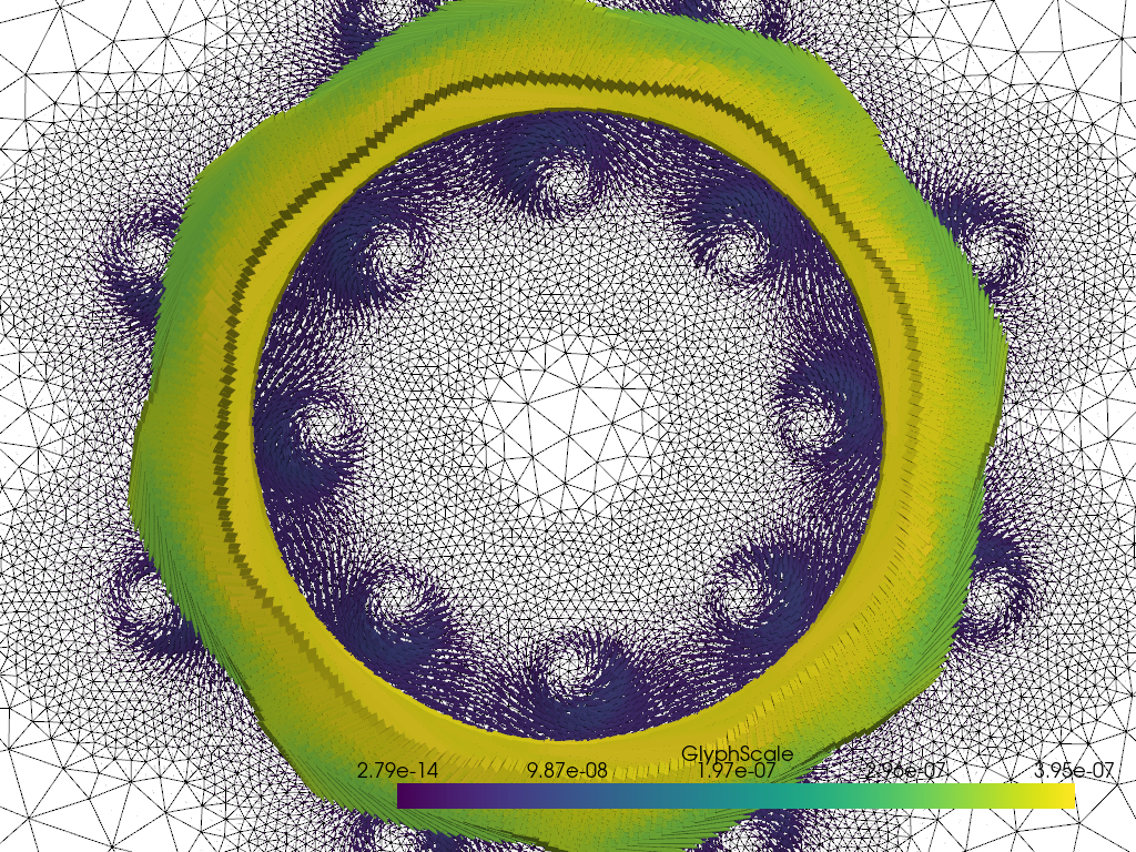
Where it fits: The most general option here, and the most work. Reach for it when the physics isn't standard solid mechanics (multiphysics, custom constitutive laws, magnetostatics) and the model is too big for scikit-fem. The example below is an iron cylinder with copper wires wound around it, solved for the magnetic vector potential A_z and the magnetic field B.

Not checked here: there are no pip wheels. Install from conda-forge (fenics-dolfinx) or the official Docker images (dolfinx/dolfinx, dolfinx/lab); on Windows that means WSL or Docker. LGPL-3.0.

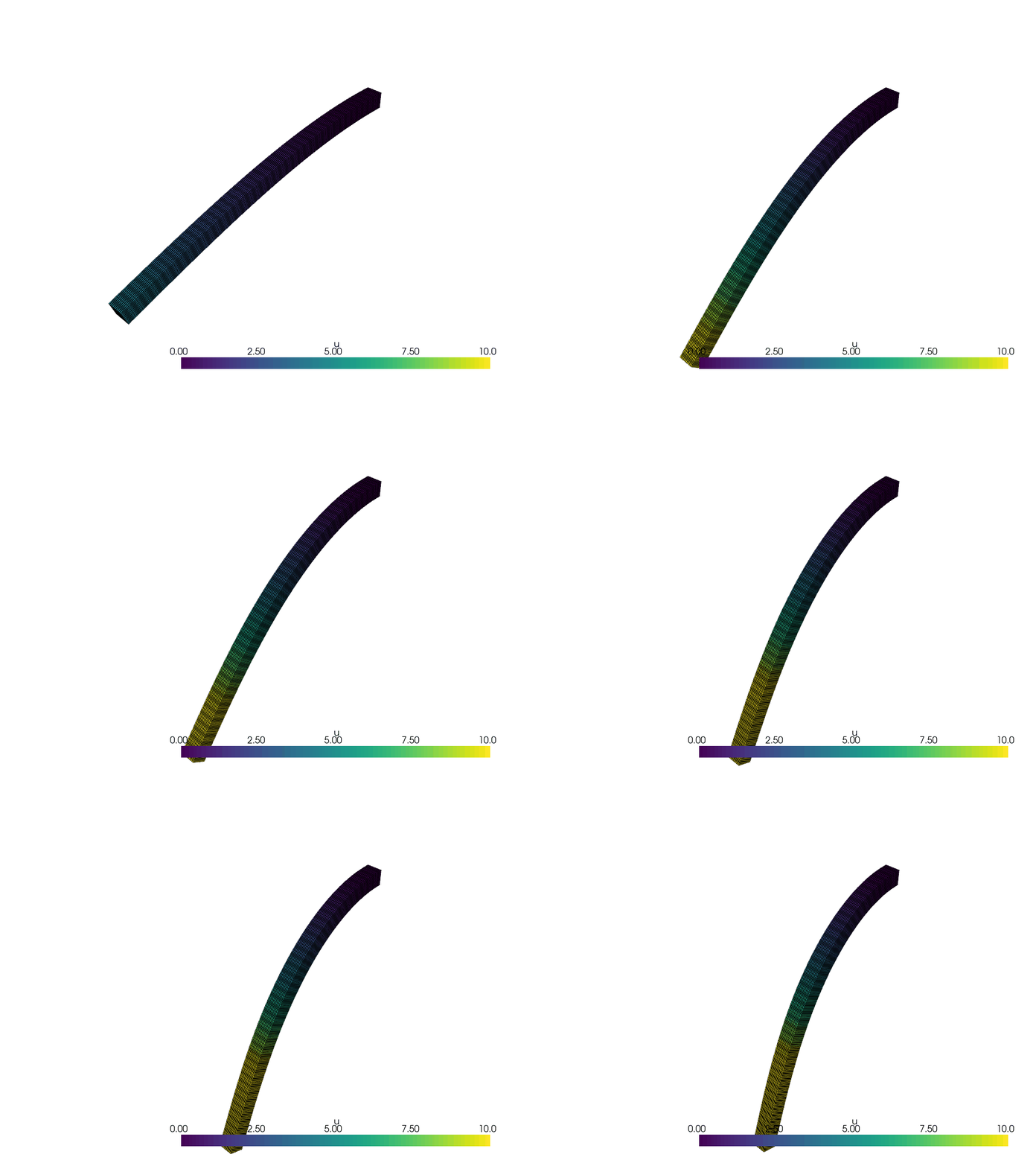_{Images: The FEniCSx tutorial by Jørgen S. Dokken, CC BY 4.0. Top row and bottom left: the Electromagnetics example; the A_z image was rendered from its interactive plot and cropped, and B is the screenshot the tutorial saves for its front-page gallery. Bottom right: the Hyperelasticity example, unchanged.}

RapidFEM

site · repo

Use for: Full-wave 3D electromagnetic FEA, in the frequency domain and the time domain: waveguides, filters, antennas and RF passives. It returns S-parameters (Touchstone), eigenmodes and far-field patterns. The core is Rust with a Python API, and prebuilt Windows wheels mean pip install rapidfem needs no compiler.

Where it fits: RF and microwave work only. It has no magnetostatic or low-frequency eddy-current solver, so coils, iron cores and motors belong in a FEniCSx model like the one above. AGPL-3.0, with commercial terms available. A young, fast-moving project.

Checked: 0.24.0. A 30 mm length of WR-90 waveguide at 8, 10 and 12 GHz gave |S₁₁| = 0.0000 and |S₂₁| = 1.0000, and an S₂₁ phase within 0.006° of TE₁₀ theory (−βL), after a constant 180° from port 2's polarity convention. Meshing and the three-frequency solve took about 3 s.

GXBeam

docs

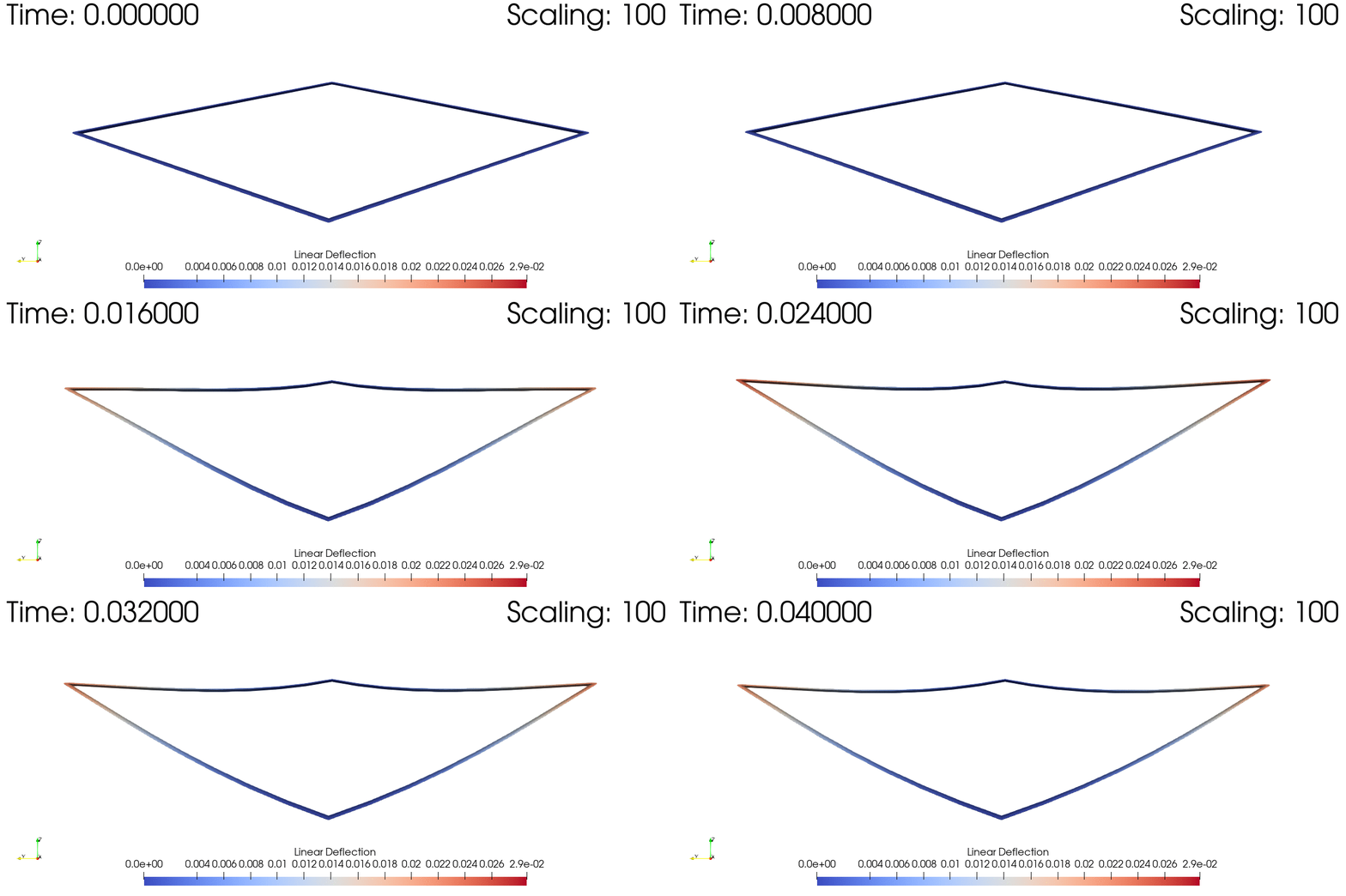
Use for: Large-deflection, very flexible structures such as wind-turbine blades and high-aspect-ratio wings, with geometrically exact beam theory. It is a Julia package, not Python, and not checked here.

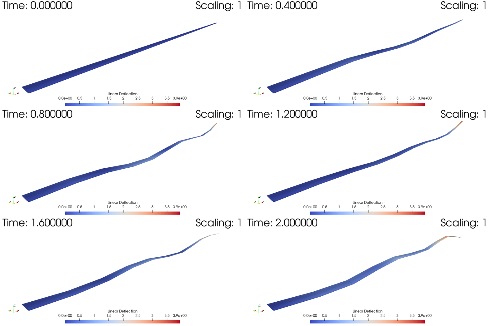_{Images: GXBeam.jl documentation, © Taylor McDonnell and contributors (BYU FLOW Lab), MIT License.}

Symbolic math and mechanisms

SymPy

docs · mechanics

Use for: Symbolic derivations: algebra, calculus, and closed forms to check a numerical answer against. Two modules do most of the design-desk work:

• sympy.physics.continuum_mechanics.beam solves beams by singularity functions, symbolically, including internal hinges (apply_rotation_hinge).
• sympy.physics.mechanics forms equations of motion for multibody systems by Kane's or Lagrange's method. Joints connect rigid bodies, and a System collects them and writes the equations. It is the core of PyDy, so there is nothing extra to install.

_{Images: SymPy documentation, © SymPy Development Team, BSD-3-Clause.}

mechanism

repo

Use for: Planar linkage kinematics (position, velocity and acceleration of four-bars, slider-cranks, engines and multi-loop linkages) from vector loop equations you write once. It also designs cam profiles, with SVAJ diagrams and pressure angle, and involute spur gears with AGMA proportions. It animates with Matplotlib and exports cam and gear coordinates for SolidWorks.

Checked: 1.1.10. A four-bar at a 60° crank angle matched the closed-form position, velocity and acceleration to 10⁻¹¹. A 60-tooth, 32-pitch gear gave d = 1.875 in, addendum 1/P, dedendum 1.25/P and base radius r cos 20°.

_{Images: mechanism README, © 2021 Gabriel Nix Morris, MIT License.}

Numerics

NumPy, pandas and Matplotlib

Everything above runs on these. NumPy is the array core, and the MATLAB replacement (see MATLAB and Simulink alternatives). pandas reads and writes Excel, CSV and JSON tables. Matplotlib draws the plots, and free-body diagrams too.

SciPy does more than most people use it for

These are the SciPy examples the rest of the page refers to. The smoke test runs each method against a closed form.

optimize.brentq: solve an implicit design equation

Size a member for a target factor of safety instead of guess-and-check. It is bracketed, so it can't wander off, which makes it the right default for monotonic design relations. Same family: root for systems, fsolve for legacy code.

shaft for n = 2.0 under M = 12 000 lbf·in, Sy = 50 kpsi
→ d = 1.6973 in   (check: n = 2.000)

optimize.curve_fit / least_squares: fit a material model to test data

Basquin S–N, Ramberg–Osgood, Paris law, creep correlations. curve_fit also returns the covariance matrix, which feeds straight into uncertainties for confidence bands on the fitted curve.

4 points of S–N data → S = 2.262e5 · N^(−0.1274)
S at 5×10⁵ cycles = 42 485 psi

integrate.quad: Castigliano without closed-form integration

When ∂U/∂P is ugly (tapered sections, curved beams, combined loading), integrate numerically. It is also the honest route to section properties of shapes with no formula.

cantilever δ = ∫ M(∂M/∂P)/EI dx
→ 3.072000 in    exact PL³/3EI = 3.072000 in

integrate.solve_ivp: transient and vibration response

SDOF and MDOF time histories, shock response, rotor run-up. dense_output=True gives a continuous interpolant you can sample anywhere afterwards. Feed the result to wetb for rainflow counting and you have a fatigue chain end to end.

m=1, c=2, k=100, x₀=0.01
→ ωn = 10.000 rad/s, ζ = 0.1000, peak |x| = 0.01000 m

linalg.eigh / eigvalsh: principal stresses in 3D

Symmetric-matrix eigensolvers give principal stresses and their directions in one call. The same routine gives natural frequencies and mode shapes from K and M. Use eigh, never the general eig, on a stress tensor: it guarantees real eigenvalues and orthogonal directions.

σx=80, τxy=50 MPa   (Shigley Ex 3-4)
→ principals [104.03, 0, −24.03] MPa   τmax = 64.03 MPa

stats.weibull_min / norm / lognorm: life scatter and reliability

Weibull is the standard fatigue-life and bearing-life model; .ppf() gives B10 / L10 directly. The natural next step after the normal-distribution statistics in Shigley Ch. 1.

shape 2.3, scale 1.2e6 → B10 life = 4.511e+05 cycles

---

MATLAB and Simulink alternatives

"A MATLAB alternative" means one of two things:

1. Running MATLAB code you already have (course scripts, a legacy calc, a toolbox written in .m files, like CALFEM's MATLAB original) needs the MATLAB language: GNU Octave.
2. Doing what MATLAB does, starting fresh is the Python stack above: NumPy, SciPy and Matplotlib, plus python-control for the Control System Toolbox.

Simulink splits too, and this split matters more:

• Causal (signal-flow) block diagrams are Simulink itself. Every block has inputs and outputs, so you derive the equations of motion first, then wire them up as integrators and gains. That suits control loops and signal processing. Free counterparts: PathSim and SimuPy in Python, and Scilab's Xcos.
• Acausal (physical-network) models are Simscape. You connect a mass, a spring and a damper at a shared flange, and the tool writes the equations. When the layout changes, nothing has to be re-derived. That suits drivetrains, hydraulics and thermal networks. Free counterparts: OpenModelica, and ModelingToolkit.jl in Julia.

A causal tool is not a Simscape replacement. The difference shows once the plant has more than a few physical parts.

Tool	Stands in for	How you model	Language	License	Install on Windows
NumPy, SciPy, Matplotlib, python-control	MATLAB and the Control System Toolbox	Scripts and notebooks	Python	BSD	pip
GNU Octave	MATLAB, the language	Scripts; most .m files run unchanged	MATLAB	GPL-3.0	installer
Scilab with Xcos	MATLAB-like numerics and Simulink-like diagrams	Scripts; causal blocks, plus a few Modelica (acausal) palettes	Scilab: MATLAB-like, not compatible	GPL-2.0	installer
PathSim	Simulink	Causal block diagram, in code or in the PathView browser editor	Python	MIT	pip
SimuPy	Simulink	Causal block diagram in code; blocks can be SymPy expressions	Python	BSD-2-Clause	pip, but the last release (2022) fails on NumPy 2
OpenModelica	Simulink with Simscape	Acausal components from the Modelica Standard Library	Modelica	AGPL-3.0 (or OSMC-PL)	installer
ModelingToolkit.jl	Simscape, as code	Acausal and symbolic	Julia	MIT core; AGPL parts since v11	Julia's package manager

FMI: how models move between these tools

FMI, the Functional Mock-up Interface, is the open standard for moving compiled simulation models between tools. An exported model, an FMU (Functional Mock-up Unit), is a zip file holding an XML description of its variables and compiled code, or C sources, that evaluate it. Wolfram's What is FMI? is a readable introduction.

The kind of FMU decides who integrates the equations:

• Model exchange: the FMU returns the state derivatives, and the importing tool integrates them with its own solver, error control included.
• Co-simulation: the FMU carries its own solver, and the importing tool only asks it to advance one communication step at a time. Its accuracy is whatever the exporting tool built in, as the figure below shows.

How the tools on this page connect:

• Out of Simulink. None of these tools opens a .slx file. Simulink can export an FMU with a Simulink Compiler license; one exported from a variable-step model also needs the free MATLAB Runtime on the machine that runs it.
• Out of OpenModelica. buildModelFMU exports any model as model exchange, co-simulation, or both. The script is in the OpenModelica section.
• Into Python. FMPy runs any FMU, and simulate_fmu("MCK.fmu") returns the result as a NumPy array, next to an independent check in the same notebook.
• Into a block diagram. pathsim-fmi wraps an FMU as a PathSim block, with ports named after its inputs and outputs, so a plant drawn acausally in OpenModelica can sit inside a causal control loop. PathSim 0.27.1 still ships the same blocks, marked deprecated in favor of the separate package.

Checked: FMPy 0.3.32 and pathsim-fmi 0.1.1, with FMI 2.0 FMUs exported by OpenModelica 1.27.1 (FMI 3.0 not tested). The m-c-k model from the OpenModelica section, run in FMPy as model exchange at a relative tolerance of 10⁻¹⁰, matches the closed-form response to 1.7 × 10⁻⁷ of x₀. The same plant, exported with a force input and a position output and placed inside a PathSim PID loop, matches python-control's closed-loop step response to 2 × 10⁻¹² m on a 10 mm setpoint. That is one plant, written acausally in Modelica, closed in a causal loop, and checked against a third tool.

_{Figure: drawn for this README from FMUs exported by OpenModelica 1.27.1 and run in FMPy 0.3.32.}

GNU Octave

site · docs · packages

Use for: Running existing MATLAB code without a MATLAB license. The syntax, matrix semantics, 1-based indexing and most core functions match MATLAB, so .m files usually run unchanged.

Where it fits: Octave is compatible with the MATLAB language, not the MATLAB product. There is no Simulink and no .slx, App Designer apps don't run, and community packages (control, signal, statistics, optim, symbolic, installed with pkg install) cover the common toolbox functions, not all of them. Use it to keep old .m code alive and to check a Python rewrite against it; for new work, the Python stack does more. From Python, oct2py calls .m functions with NumPy arrays both ways, so the original and the rewrite can run on the same inputs in one notebook. GPL-3.0. The current release is 11.3 (June 2026); Ubuntu 24.04's apt still ships 8.4.

Checked: Octave 8.4.0 with its control package 4.0.1, and oct2py 6.1.1. The CALFEM cantilever, run through CALFEM's original MATLAB code (calfem-matlab, unmodified) from Python, assembles a K identical, entry for entry, to the one the Python port builds. The displacements agree with the port's to 1 × 10⁻¹⁵: a tip deflection of 25.600 mm and wall reactions of 1000 N and 2000 N·m. For the m-c-k system in the SciPy examples above, damp(tf(1, [1 2 100])) gives ωn = 10 rad/s and ζ = 0.1, and step on a fine time grid gives a 72.925% overshoot, matching exp(−πζ/√(1−ζ²)).

The MATLAB original's API differs from the Python port's in two places, so a line-by-line translation breaks:

Edof = [1  1 2 3  4 5 6;    % element number first, then its DOFs.
        2  4 5 6  7 8 9];   % Python's edof has no element-number column
bc = [1 0; 2 0; 3 0];       % [DOF, prescribed value]. Python's solveq takes only the DOFs

PathSim

site · docs · repo · editor

Use for: Simulink-style block diagrams in plain Python: integrators, gains, transfer functions, state-space and PID blocks, discrete-time blocks and scopes, for continuous, discrete and hybrid systems. Zero-crossing events cover impacts, switches and relays. About 30 ODE solvers come with it, including adaptive (RKDP54, RKF78) and implicit ones for stiff systems (ESDIRK, BDF). PathView, its browser editor, builds the same diagrams by drag-and-drop and exports them as PathSim scripts.

Where it fits: Control loops and signal flow, once a model has several interacting parts you want to swap or mixes discrete and continuous time. For a single ODE, solve_ivp takes less code. It is causal, so it stands in for Simulink, not Simscape: you derive the equations yourself, as in the snippet. MIT license, described in a 2025 JOSS paper. It is pre-1.0 and moving fast, from 0.20 in March 2026 to 0.27 in October, so keep it pinned.

Checked: 0.27.1. The snippet runs the m-c-k system from the SciPy examples, released from x₀ = 10 mm. With the adaptive RKDP54 solver it matches the closed-form damped response to 3.6 × 10⁻⁹ of x₀. With the default solver the error is 6.2 × 10⁻³ of x₀ (see the figure, and the gotchas). A PID loop around the same plant matches python-control's closed-loop step response to 5 × 10⁻¹⁰ m on a 10 mm setpoint.

_{Figure: drawn for this README from two runs of the snippet below, one with PathSim's default solver and one with RKDP54.}

The snippet: the m-c-k system as a block diagram

from pathsim import Simulation, Connection
from pathsim.blocks import Integrator, Amplifier, Adder, Scope
from pathsim.solvers import RKDP54

m, c, k = 1.0, 2.0, 100.0          # [kg, N·s/m, N/m]

v = Integrator(0.0)                # velocity [m/s], v(0) = 0
x = Integrator(0.01)               # displacement [m], x(0) = 10 mm
damp = Amplifier(-c / m)
spring = Amplifier(-k / m)
acc = Adder()                      # x'' = -(c/m) x' - (k/m) x
scope = Scope()

sim = Simulation(
    blocks=[v, x, damp, spring, acc, scope],
    connections=[
        Connection(v, x, damp),    # one output, several inputs
        Connection(x, spring, scope),
        Connection(damp, acc[0]),
        Connection(spring, acc[1]),
        Connection(acc, v),
    ],
    Solver=RKDP54,                 # the default is fixed-step, 2nd order
    tolerance_lte_rel=1e-8,
    tolerance_lte_abs=1e-12,
    log=False,                     # it logs progress to the console by default
)
sim.run(3.0)                       # simulate 3 s
t, (xs,) = scope.read()            # time [s], displacement [m]

SimuPy

repo · docs

What it is: Simulink-style block diagrams built on state-space systems, with one real strength: blocks can be SymPy expressions, so equations of motion derived with sympy.physics.mechanics go straight into a diagram, with no hand transcription. A block with state also can't pass its input straight to its output, so a diagram can never contain an algebraic loop. BSD-2-Clause. NASA's SimuPy Flight Vehicle Toolkit is built on it.

Why it isn't in requirements.txt: the code hasn't kept up with NumPy or SymPy. The last release, 1.1.2 from May 2022, uses np.Inf, which NumPy 2.0 removed, yet pip check reports nothing wrong, because SimuPy declares numpy>=1.11.3 with no upper bound. The fix was merged on GitHub in May 2026 and never released. Even from that commit, the symbolic API, the main reason to choose SimuPy, fails on SymPy 1.14, and the project's own test suite gives 20 failures and 3 errors. A 2022 stack (NumPy 1.23, SciPy 1.9, SymPy 1.10) gives the same counts, so the failures predate NumPy 2. The NASA toolkit pins numpy<2, and its last commit was in December 2024.

Checked: the numeric API, installed from the merged commit (1c2c43a). The m-c-k free vibration from the PathSim section matches the closed form to 3.7 × 10⁻⁷ of x₀ with the default solver, dopri5 at a relative tolerance of 10⁻⁶. A tighter tolerance needs a larger nsteps as well; see the gotchas.

Use PathSim for new work. To run an existing SimuPy model, give it its own NumPy 1.x environment, and check it against a closed form before trusting it, because its own tests fail there too.

SimuPy and PathSim compared. Both are causal, so both stand in for Simulink, not Simscape.

	SimuPy	PathSim
How a diagram is solved	One state vector for the whole diagram, integrated by one SciPy solver	Each block keeps its own state, and one of PathSim's solvers advances all of them
Algebraic loops	Impossible by design. A PID's proportional path needs its own stateless block	Detected and solved by iteration
Symbolic models	Blocks can be SymPy expressions (broken on current SymPy, above)	None; blocks are NumPy code
Stiff systems	Not supported. Only SciPy's dopri5 and dop853 give the step callback SimuPy needs	Implicit ESDIRK and BDF methods, among about 30 solvers
Events	Zero-crossing events and switched systems	Zero-crossing, scheduled and conditional events
Releases	1.1.2, May 2022, the last	87 since August 2024; 0.27.1 in October 2026

python-control

docs · repo

Use for: What MATLAB's Control System Toolbox does: transfer-function and state-space models, feedback connections, step and frequency responses, Bode, Nyquist and root-locus plots, gain and phase margins, pole placement, LQR, and continuous-to-discrete conversion. control.matlab provides the MATLAB names (tf, ss, step, bode, lsim, margin), so a MATLAB script ports almost line for line. Install and import it as control (import control as ct). BSD-3-Clause.

Where it fits: Linear analysis and controller design. Pair it with PathSim for the time response of the nonlinear or hybrid system the linear design is for, and use each to check the other.

Checked: 0.10.2, without the optional Slycot (LQR, Kalman gains, pole placement and sample_system all work without it). For the m-c-k system, damp gives ωn = 10 rad/s and ζ = 0.1, and dcgain gives 1/k = 0.01 m/N. A step response on a fine time grid overshoots by 72.92476%, as exp(−πζ/√(1−ζ²)) predicts. Its closed-loop step response for the PID loop above is the reference PathSim was checked against.

OpenModelica

site · docs

Use for: Acausal physical modeling, the free counterpart to Simscape and to commercial Modelica tools such as Dymola. You connect components from the Modelica Standard Library (translational and rotational mechanics, multibody, electrical, thermal, fluids) in the OMEdit editor or as Modelica text, and OpenModelica derives and solves the equations. It exports and imports FMUs, and OMPython drives it from Python.

Where it fits: Physical systems you would rather draw than derive: a drivetrain with a clutch, a hydraulic circuit, a thermal network, an electromechanical actuator. The m-c-k system below is four components and four connect statements, with no equation written by hand; in PathSim you write x'' = −(c/m)x' − (k/m)x first. AGPL-3.0 for anyone, or the OSMC-PL for members of the consortium behind it; the Modelica Standard Library is BSD-3-Clause. The current release is 1.27.1 (September 2026).

Install: a standalone program, not a pip package: the Windows installer, or the apt repository or Docker images on Linux (the -minimal image holds the compiler only). Get the Standard Library with installPackage(Modelica), or point setModelicaPath at a clone of the ModelicaStandardLibrary repository. OMPython, which is pinned, needs OpenModelica's omc running locally or in a container. omc refuses to serve OMPython's ZeroMQ connection as root, so give a container a --user.

Checked: 1.27.1 with Modelica Standard Library 4.1.0, in the official Docker image on Linux. checkModel reports 23 equations in 23 variables for the model below, 13 of them trivial, and none written by hand. Simulated with DASSL at a tolerance of 10⁻¹⁰, it matches the closed-form response to 1.1 × 10⁻⁷ of x₀. OMPython 4.1.0, on the host, drove the same OpenModelica through ZeroMQ and got the same result. The FMUs from the export script are the ones checked in the FMI section.

model MCK "Mass on a spring and damper, released from x0 = 10 mm"
  import TC = Modelica.Mechanics.Translational.Components;
  TC.Fixed fixed;
  TC.Spring spring(c = 100) "N/m";
  TC.Damper damper(d = 2) "N.s/m";
  TC.Mass mass(m = 1, s(start = 0.01, fixed = true), v(start = 0, fixed = true)) "kg";
equation
  connect(fixed.flange, spring.flange_a);
  connect(fixed.flange, damper.flange_a);
  connect(spring.flange_b, mass.flange_a);
  connect(damper.flange_b, mass.flange_a);
end MCK;

To export it as an FMU, run omc export.mos with this script:

loadFile("MCK.mo");
setCommandLineOptions("--fmiFlags=s:cvode");  // without it, co-simulation steps with explicit Euler
buildModelFMU(MCK, version = "2.0", fmuType = "me_cs");

---

Gotchas

Traps found while checking the packages above. Many run without an error and give a wrong answer, which is why every result here gets an independent check.

handcalcs, units and PDF export

• handcalcs prints pint's canonical unit names. It ignores the registry formatter, so 12 * u.kpsi renders as kilopound_force_per_square_inch. Define short units instead: u.define("ksi = 1000 * pound_force / inch ** 2") renders as ksi.
• Keep %%render cells to plain assignments. .to() and print() inside a rendered cell won't render; do those in a normal cell.
• No underscores or ^ in handcalcs comments. Each comment goes inside \textrm{...}, where an underscore is illegal. MathJax (classic Jupyter, Colab) tolerates it, but KaTeX, which VS Code uses, throws ParseError: Expected 'EOF', got '_' and the whole cell fails to render. Write # bore radius, not # r_i is the bore; subscripts belong in the variable names.
• pint's micro prefix also breaks KaTeX. pint writes it as the micro sign (U+00B5), so a result in microradian renders as \mathrm{µrad}. KaTeX has no glyph for that character and warns, and the symbol may not show. The Greek letter (U+03BC) works. Define a unit that uses it: u.define("microrad_greek = 1e-6 * radian = μrad"). For SI units, handcalcs.set_option("preferred_string_formatter", "~L") gives the short symbols (N, mm, MPa) without any defines.
• forallpeople 3.0.0 ships no unit environments in this build, and is SI-centric. Use pint for imperial work.
• nbconvert --to webpdf fails on Windows with a bare NotImplementedError from asyncio … _make_subprocess_transport. nbconvert switches asyncio to the Selector event loop on Windows, and Playwright needs the Proactor loop to launch its browser. It's an nbconvert bug, not a broken install. This one-liner is the normal command line with the switch turned off (checked with nbconvert 7.17.1 and Playwright 1.63): python -c "import asyncio, nbconvert.nbconvertapp as a; asyncio.set_event_loop_policy = lambda p: None; a.main()" --to webpdf "X.ipynb"
• Playwright inside a Jupyter notebook fails the same way on Windows, because ipykernel makes the same switch, and the sync API won't run inside the kernel's loop anyway. Run the async API on a fresh Proactor loop in a worker thread. Plain .py scripts need neither fix.

  import asyncio, concurrent.futures
  
  def run_playwright(coro_fn, *args):
      def runner():
          loop = asyncio.ProactorEventLoop()
          try:
              return loop.run_until_complete(coro_fn(*args))
          finally:
              loop.close()
      with concurrent.futures.ThreadPoolExecutor(1) as pool:
          return pool.submit(runner).result()

Beam solvers: sign conventions

Each package has its own signs, and none says so in an error. The textbooks (Shigley Fig. 3-3, Hibbeler Fig. 6-3) take a sagging moment as positive, so a cantilever's wall moment is negative. Checked on the worked example's cantilever, with planesections 1.4.2 and anaStruct 1.7.0:

• PlaneSections' getBMD() is hogging-positive. It returns +3645 N·m at the wall. Negate it, and pass scale=-1 to ps.plotMoment to draw the diagram the textbook way up. Its shear, deflection and rotation already follow the textbook's signs.
• PlaneSections' getSFD() and getBMD() return each node twice (left value, right value), so index 0 is the baseline, not the value at x = 0. Take [1::2]. ps.getVertDisp() returns (disp, x), displacement first; unpacking it the other way round silently gives the x coordinates.
• anaStruct reports reactions opposite to the loads that cause them. A downward load gives an upward reaction reported as negative.
• anaStruct's element shear Q and moment M are both opposite to the textbook's for elements drawn left to right, and get_node_results_system() gives node uy positive downward.

Flip the signs, then compare signed values with the closed form, not magnitudes: a magnitude check passes a wrong sign.

Stiffness matrices: CALFEM and MATLAB ports

• CALFEM installs as calfem-python but imports as calfem (import calfem.core as cfc). pip install calfem fails, because no package has that name.
• CALFEM numbers DOFs from 1, as its MATLAB original does, in edof and in the support list for solveq. A 0-based list raises no error, because index −1 wraps around to the last DOF. In the CALFEM cantilever, bc = [0, 1, 2] fixes DOFs 9, 1 and 2 instead of 1, 2 and 3: a beam pinned at the wall with its tip rotation locked. Its tip still deflects 25.6 mm, so the deflection check passes. The reactions give it away: the 2000 N·m moment appears at the tip, not the wall.
• CALFEM's eigen uses the general scipy.linalg.eig and silently drops imaginary parts. On a correctly assembled K and M it matches eigh, but it would also hide an asymmetric K, and it doesn't guarantee orthogonal mode shapes when two frequencies coincide. Use scipy.linalg.eigh on the supported K and M. (In 3.6.16, beam2de also prints its inputs on every call.)
• Translate MATLAB's eig(K) as eigh, not eig. MATLAB and Octave check whether the matrix is exactly symmetric and, if it is, use the symmetric solver, so there eig(K) and eig(K, M) return real eigenvalues and orthogonal mode shapes. scipy.linalg.eig never makes that switch. (The MATLAB check is exact: a K symmetric only to round-off takes the general path there too.)

scikit-fem

• lame_parameters(E, ν) makes a 2D model plane strain. It returns the three-dimensional λ and μ: right for a long cylinder, wrong for a thin plate, which needs plane_stress(E, ν). Modeled as a 2D solid 50 mm thick, the 2 m cantilever from the CALFEM section deflects 25.600 mm in plane stress and 23.286 mm with lame_parameters: 9% too stiff (a factor of 1 − ν²), with no warning.
• plane_stress changed meaning in 12.0.2, a patch release. Up to 12.0.1 it returned an equivalent E and ν, for linear_elasticity(*lame_parameters(*plane_stress(E, nu))). From 12.0.2 it returns λ and μ, for linear_elasticity(*plane_stress(E, nu)). Either idiom on the other version runs without error and puts displacements out by a factor of 10¹¹ or more. That error is loud, but only a check catches it. requirements.txt pins 12.0.2.

CalculiX

• Plane-stress elements are 3D slabs. CalculiX expands each CPS6 into wedges of the section thickness, with free faces, so a thick section gives a 3D answer, not the plane-stress one. For a 25 mm hole in a 100 mm plate, a 25 mm section gives K_t = 2.471, against 2.432 for a 1 mm section on the same mesh (+1.6%). Set ν = 0 and the thick section gives 2.430 again. Nothing warns, and the plane-stress K_t on Shigley's charts needs a section thin compared with the hole (t/r ≈ 0.1 or less).
• B32 beams are too stiff with few elements, and converge at about first order. On the 2 m cantilever, 10 elements give a tip deflection 1.3% low and a buckling load 0.9% high. 40 elements leave 0.31% and 0.15%. Each doubling roughly halves the error, so run an element study.
• B32 includes shear deformation. Compare it with Timoshenko, not PL³/3EI. On a slender beam the difference hides inside the mesh error. On a short one (L/h = 3) it is 8.7%.
• Stresses go only to the .frd file. *NODE PRINT takes U and RF. With S it warns "label not applicable" and leaves the .dat empty. Use *NODE FILE with S, and parse the .frd by its fixed 12-character fields.
• Gmsh's 10-node tetrahedron numbers its last two mid-edge nodes the other way round from C3D10. Swap columns 8 and 9 before writing the elements. With the wrong order the model still solves, but the stiffness is visibly wrong.

Time-domain simulation

• PathSim's default solver is fixed-step and 2nd order (SSPRK22 at dt = 0.01 s). Simulink's default is variable-step, so a model carried across keeps running, gives no warning, and loses accuracy. With ζ = 0.1, the m-c-k model's peak error is 0.6% of x₀ at ωn = 10 rad/s, 16% at 50 rad/s and 90% at 100 rad/s. Pass an adaptive solver and tolerances (Solver=RKDP54, tolerance_lte_rel, tolerance_lte_abs), or at least halve dt and see whether the answer moves.
• PathSim's PID(f_max=...) is in rad/s, not Hz. The derivative term is Kd·s/(1 + s/f_max), so its filter pole sits at f_max rad/s. The block's own docstring calls f_max=1e3 "cutoff at 1kHz"; that corner is at 159 Hz.
• OpenModelica's co-simulation FMUs step with explicit Euler by default. Unless the model is exported with --fmiFlags=s:cvode, the FMU takes one Euler step per communication interval, with no error control and no warning, and a tolerance passed by the importing tool changes nothing. For the m-c-k system the error is 8.2% of x₀ at a 4 ms step, 1.9% at 1 ms and 0.19% at 0.1 ms: first order. Exported with the flag, it is 4.7 × 10⁻⁶ at 4 ms. Model exchange avoids the question, because the importing tool integrates. The FMU's own source says it: with no flags file, it falls back to S_EULER.
• FMPy's default tolerance comes from the FMU's default experiment, 10⁻⁶ in OpenModelica's export. That left the model-exchange m-c-k run 6 × 10⁻⁴ of x₀ off. Pass relative_tolerance to simulate_fmu.
• SimuPy returns a truncated result when its solver runs out of steps. The default nsteps = 500 caps the solver's steps between events, and a tight rtol uses it up. SimuPy warns Integrator quit unsuccessfully and returns the trajectory so far: asked for 3 s of m-c-k at rtol = 1e-10, it returned 1.51 s. An error check over the returned points still passes. Check res.t[-1], and raise nsteps with the tolerance.
• python-control's step_info measures on its own coarse time grid. For the m-c-k system it takes 276 points over 6.9 s, steps over the peak, and reports a 72.50% overshoot where theory gives 72.92%. Pass T=np.linspace(0, t_end, n) fine enough to resolve the peak. forced_response also needs evenly spaced times, and raises an error otherwise.

---

License

MIT, for the documents and code written for this repository. See LICENSE.

Images from other sources keep their own licenses, credited under each one above. The worked example's problem figure, assets/cantilever-triangular-load.png, was drawn for this repository and is covered by the MIT license; the problem itself follows R. C. Hibbeler, Mechanics of Materials, 8th ed., Example 1.1 (Fig. 1–4), credited in the notebook.