kirchcig

GPU Kirchhoff migration to common-image gathers (CIGs), with an exact adjoint.

English | 简体中文

Hand-written CUDA kernels, compiled at runtime by NVRTC through CuPy. PyTorch is an optional zero-copy autograd adapter, not part of the compute path.

Install

pip install "kirchcig[cuda12]"     # GPU, CUDA 12.x
pip install "kirchcig[cuda11]"     # GPU, CUDA 11.x
pip install kirchcig               # CPU only, NumPy reference engine

No compiler and no nvcc needed; kernels are built at runtime by NVRTC.

Extra	Pulls in	Gives you
(none)	numpy	engine="numpy", the reference engine. Runs anywhere, slow.
cuda12 / cuda11	cupy-cuda12x / cupy-cuda11x	engine="cuda", the GPU engine. Pick the one matching your driver.
eikonal	scikit-fmm	Traveltimes for a non-constant velocity model.
torch	torch	kirchcig.torch, the autograd wrapper.
test	pytest, scipy, scikit-fmm	Test suite, and op.to_scipy().

Combine them: pip install "kirchcig[cuda12,eikonal,torch]".

Quick start

import numpy as np
from kirchcig import migrate

# data  (ns, nr, nt)   prestack traces
# vel   (nx, nz)       smooth migration velocity [m/s]
# srcs  (2, ns)        source positions, rows are (x, z) [m]
# recs  (2, nr)        receiver positions, rows are (x, z) [m]

cig = migrate(
    data, vel, srcs, recs,
    dt=0.004, dx=10.0, dz=10.0,
    nh=32, hmax=2000.0,        # 32 half-offset bins out to 2000 m
)
# cig -> (32, nx, nz)

image = cig.sum(0)             # (nx, nz) stacked image; nh=1 gives it directly

No data at hand? This runs out of the box:

from kirchcig import KirchhoffCIG
op = KirchhoffCIG.demo()       # constant velocity, one point scatterer
assert op.dot_test()
cig = op.adjoint(op.demo_data())

Usage

The operator pair

For inversion you want the operator, not the one-shot function:

from kirchcig import KirchhoffCIG

op = KirchhoffCIG(
    nx=401, nz=201, dx=10.0, dz=10.0,
    srcs=srcs, recs=recs,
    nt=1500, dt=0.004,
    vel=vel,
    nh=32, hmax=2000.0,
    domain="offset",           # or "angle"
    engine="cuda",             # or "numpy", "auto"
)

cig  = op.adjoint(data)        # (ns, nr, nt) -> (nh, nx, nz)   migration
data = op.forward(cig)         # (nh, nx, nz) -> (ns, nr, nt)   demigration
op.dot_test()                  # True

forward and adjoint are exact transposes to accumulator precision, so they drop into any least-squares solver:

import scipy.sparse.linalg as spla
cig_lsm = spla.lsqr(op.to_scipy(), data.ravel(), iter_lim=20)[0].reshape(op.shape_model)

Angle-domain gathers

op = KirchhoffCIG(..., domain="angle", nh=30, hmax=60.0)   # 30 bins, 0-60 deg

hmax is the maximum half opening angle in degrees. Bin indices come from source- and receiver-side emergence angles, computed from the traveltime gradients.

Anti-alias filtering

op = KirchhoffCIG(..., aa=True)                 # default aa_factor=1.0, aa_max=32

Kirchhoff summation aliases wherever the operator's moveout between neighbouring traces exceeds half a period of the highest frequency present. It shows up as steeply dipping, criss-crossing arcs at large offsets and shallow depths; on coarsely sampled data they dominate the image. aa=True reads every contribution through a triangle filter whose half-width follows the local operator dip, the standard remedy of Lumley, Claerbout and Bevc (1994) as used by Claerbout's trimo and Madagascar's sfmig2.

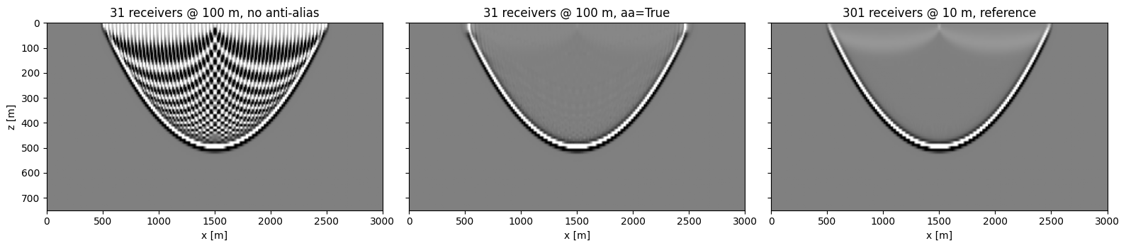
_{One shot, a band-limited spike in every trace. Left: 31 receivers at 100 m, plain summation. Middle: the same data with aa=True. Right: 301 receivers at 10 m, no filter. python examples/antialias.py.}

• aa_factor scales the filter width and is the antialias= parameter of trimo and sfmig2 (all default to 1.0). 2.0 puts the triangle's first spectral null exactly on the alias frequency, at the cost of resolution on steep dips.
• aa_max caps the half-width in samples (default 32).
• aa_stretch (default on) also covers the time footprint of the image cell, |dtau/dx| dx + |dtau/dz| dz. An image sample stands for a dx * dz cell; when the depth grid is coarser than the time sampling (2 dz / v > dt) each depth sample of a plain summation lands several time samples apart and a demigrated reflector is a comb of interpolated spikes. This is Madagascar's aastretch. The source and receiver gradients are summed before the absolute value, so the footprint is only the depth term at the specular point, and the two widths combine as a root mean square. The gradient rides in the traveltime-table element (16 bytes per image point in the offset domain, 32 with angles or weights); aa_stretch=False gives the pure trace-axis criterion of sfmig2.
• Operator dips come from differencing the traveltime tables along the trace axis, so it works for eikonal and user-supplied tables alike. The source and receiver axes must be sorted along the line; the constructor warns otherwise.
• The operator pair stays an exact transpose; dot_test() passes with the filter on.
• Cost: the filter is applied through a three-tap identity on the double integral of the traces, so the price does not depend on the filter width. It does need a float64 copy of the data, ns * nr * (nt + 2*aa_max + 1) * 8 bytes, and the adjoint reads three float64 taps per contribution instead of one float32 sample. On a V100 that is 1.8x on the adjoint and 2.8x on the forward (see Performance); python benchmarks/bench.py --aa measures it on yours.

Migration aperture

op = KirchhoffCIG(..., aperture=60.0)           # cone half-angle from the vertical [deg]
op = KirchhoffCIG(..., apt=3000.0)              # or a lateral distance [m]; both may be combined

A trace contributes to an image point only if the point lies inside the aperture of both its source and its receiver: within aperture degrees of the vertical below them (sfkirmig's aperture=), or within apt metres laterally (sfmig2's apt=, in metres here). This suppresses far-aperture swing noise and skips the dropped contributions' work. On the README geometry a 60-degree cone keeps 47% of the trace-image-point pairs (45 degrees: 23%); on the V100 that cut the forward from 25.5 to 17.2 ms while the adjoint did not speed up at all, because its blocks are depth columns that straddle the cone edge, so masked lanes idle while their warp-mates gather and the coalesced table read is still made for every pair. Treat the aperture as an imaging control that comes with a forward speed-up. The cut is hard, as in Madagascar; op.aperture_masks() returns the two boolean masks, python benchmarks/bench.py --aperture 60 prints the kept fraction and the timing.

The aperture is applied on the host by pushing the masked traveltime-table entries past the end of the trace, where the kernels already skip. No kernel changes, both engines drop exactly the same contributions, and the pair stays an exact transpose.

Amplitude weights

op = KirchhoffCIG(..., weight="obliquity")                     # sqrt(cos theta) per side
op = KirchhoffCIG(..., weight=["obliquity", "spreading"])      # times 1/sqrt(t) per side
op = KirchhoffCIG(..., weight=lambda t, theta, dt: np.cos(theta) ** 2)
op = KirchhoffCIG(..., weight=(w_srcs, w_recs))                # (ns, nx, nz), (nr, nx, nz)

Every contribution is multiplied by w_s(src, x, z) * w_r(rec, x, z), the product of a source-side and a receiver-side table. Presets are "obliquity" (sqrt(cos theta), the product is the geometric mean of the two emergence cosines, the obliquity factor of Kirchhoff modelling; sfkirmod uses the arithmetic mean, which agrees to second order) and "spreading" (1 / sqrt(t), the 2D Green's function amplitude of one leg up to the velocity); a list multiplies them; a callable is evaluated on each side's traveltime and emergence-angle tables; a pair of arrays is used as is. Both kernels multiply by the same float32 product, so forward is A W, adjoint is W A^T and the pair stays an exact transpose. The weight rides in the traveltime-table element, so it costs no extra memory transaction. These cover the obliquity and spreading factors; the full true-amplitude (Bleistein) weights are not separable into two sides and are not provided.

Half-derivative (rho) filter

op = KirchhoffCIG(..., halfderiv=True)

Kirchhoff demigration in 2D needs a half-order time derivative. Spreading each image point along its traveltime curve and summing the spread points over a reflector leaves the stationary-phase factor of the one lateral integral behind: a 45-degree phase rotation and an |omega|^-1/2 spectral tilt. A demigrated horizontal reflector then does not return the wavelet it was built with, and a migrated one carries the rotation the other way. halfderiv=True applies H(omega) = sqrt(1 - rho e^{-i omega}), the half of the backward difference, to every trace on the way out of forward and its exact transpose to the data on the way into adjoint. It is the filter Madagascar's sf_halfint implements and sfmig2, sfkirchnew and sfkirmod apply, with the same default leak rho = 1 - 1/nt; halfderiv_rho changes it.

It costs one float64 FFT per trace, runs on the engine's device, and is independent of the kernels. dot_test() passes with it on. Two properties to know: the discrete filter delays by a quarter sample (its phase is pi/4 - omega/4), so migrated reflectors sit dt/4 shallower in two-way time and round trips are unshifted; and it does nothing about the depth-grid comb (2 dz / v > dt), which is what aa=True handles.

PyTorch

from kirchcig.torch import TorchKirchhoffCIG

top = TorchKirchhoffCIG(op)
cig = top.adjoint(data)        # differentiable w.r.t. data
res = top.forward(cig) - data
res.pow(2).sum().backward()

Tensors stay on the GPU. The operator is linear, so the backward of forward is adjoint and vice versa; the backward pass is itself recorded, so second-order derivatives work.

Custom traveltimes

op = KirchhoffCIG(..., trav=(trav_srcs, trav_recs))
# trav_srcs (ns, nx, nz)   source-to-image-point traveltimes [s]
# trav_recs (nr, nx, nz)   image-point-to-receiver traveltimes [s]

Otherwise traveltimes come from an eikonal solve (scikit-fmm), or analytically for constant velocity. Note the layout: the source/receiver axis comes first, transposed relative to some other libraries, which is what keeps the adjoint reads coalesced.

Shapes

	Shape	Notes
data	(ns, nr, nt)	float32
model (CIG)	(nh, nx, nz)	gather axis outermost
srcs, recs	(2, ns), (2, nr)	rows are (x, z) in metres
velocity	(nx, nz) or scalar	m/s

Examples

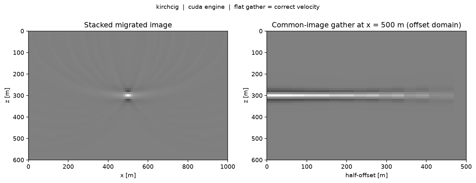
python examples/plot_cig.py          # the cover figure
python examples/vel_analysis.py      # the figure below
python examples/antialias.py         # the anti-aliasing figure above
python examples/lsqr_migration.py    # least-squares migration with SciPy LSQR
python examples/torch_deep_prior.py  # deep-prior LSM
python benchmarks/bench.py           # timings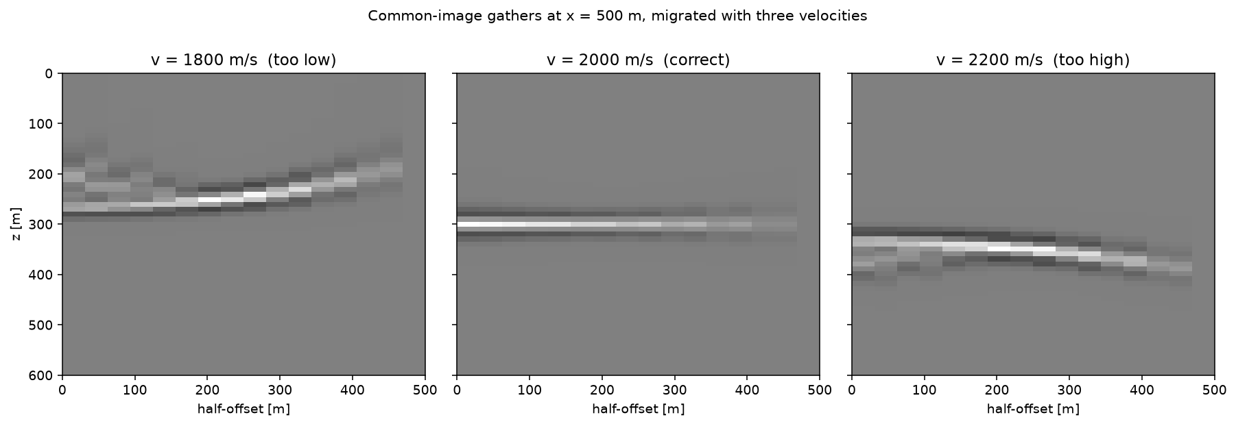

_{The same data migrated with three velocities. Flat gathers mean the velocity is right; curvature along the offset axis is what migration velocity analysis measures, and stacking destroys it.}

Performance

Single Tesla V100-PCIE-32GB (driver 580.178.04), nx=401, nz=201, ns=100, nr=200, nt=1500, nh=32, offset domain. Each operator application evaluates 1.6e9 trace-image-point pairs.

Accumulator	adjoint (migration)	forward (demigration)	dot-test relative error
float64 (default)	33.9 ms — 47.5 G pair-evals/s	25.6 ms — 63.0 G pair-evals/s	9.5e-08
float32 *	33.5 ms — 48.2 G pair-evals/s	18.8 ms — 85.8 G pair-evals/s	1.1e-07
float64, aa=True, aa_stretch=False	72.7 ms — 22.2 G pair-evals/s	67.3 ms — 23.9 G pair-evals/s	2.0e-08
float64, aa=True (with aa_stretch)	62.0 ms — 26.0 G pair-evals/s	71.2 ms — 22.6 G pair-evals/s	2.3e-08

_{* the float32 row has not been re-timed since the adjoint started chunking its source loop, which moved every other adjoint number here; the float64 rows are the current ones.}

Building the operator, including traveltime tables and the one-off NVRTC compile, takes about 1.4 s, 2.1 s with aa=True, and 2.6 s with aa_stretch as well (the extra work is differencing the tables for the operator dips). Anti-aliasing costs 1.8x on the adjoint (three float64 taps per contribution instead of one float32 sample) and 2.8x on the forward (six shared-memory atomics instead of two, plus the float64 output and its reverse integration). Timings on this machine vary by up to 25% between sessions (the aa_stretch=False row measured 98.5 ms on another day), so compare rows measured together. forward used to be about twice as fast as adjoint — it accumulates one trace per block in shared memory and writes it out once, while adjoint does an irregular gather along the traveltime curves — but chunking the adjoint's source loop closed most of that gap, and under aa=True the forward is now the slower of the two.

--schunk sets how many sources the adjoint keeps in registers, so that each receiver-table element is read once per chunk instead of once per source. Sweeping the last row within one session: 118.1 ms at --schunk 1, 62.0 ms at the default 4, 59.5 ms at 8, with the forward untouched at 71.1 ms. That 1.9x is most of what took this row from the 128.8 ms it cost in 0.2.0; packing the gradients into the traveltime element is the smaller part of the change (128.8 to 118.1 ms at --schunk 1, measured a session apart). One result here is not explained: with both in place, aa_stretch comes out faster than the plain trace-axis filter — 62.0 against 72.7 ms — although its table element is twice as wide, and the aa_stretch=False row has not itself been swept over schunk. Until it is, read the two aa=True adjoint numbers as about equal rather than as a measured cost of the stretch term.

The angle domain pads the element to its widest, 8 floats: traveltime, emergence angle, operator dip and both gradient components. --domain angle --aa costs 91.1 ms on the adjoint and 113.7 ms on the forward in the same session, with a dot-test error of 8.4e-08.

float64 accumulation is close to free on Volta and other data-centre cards (1:2 FP64:FP32) and buys bit-identical agreement with the NumPy reference engine. On consumer GeForce parts the ratio is about 1:64, so acc="float32" is the sensible default there; it costs roughly 1e-7 of relative accuracy.

Reproduce with python benchmarks/bench.py; --acc float32, --nh, --domain, --aa, --no_aa_stretch, --aperture, --halfderiv, --weight, --schunk and --engine numpy are accepted. The first two rows are without anti-aliasing. The operator runs on one device; select it with cupy.cuda.Device, or from the PyTorch wrapper by the tensor's device.

How it works

The kernels live as a CUDA C++ string in kirchcig/_kernels.py, compiled by cupy.RawKernel(..., backend="nvrtc") on first use and cached by CuPy afterwards. CuPy only allocates memory, compiles and launches; all arithmetic is in the kernels.

• Why hand-written. Kirchhoff migration is an irregular gather along traveltime curves, not a matmul or a convolution. No tensor op expresses it without blowing up memory traffic, and writing the kernel directly is what makes the rest of this list possible.
• No atomics in the adjoint. One thread per image point owns the whole gather axis, so every write is exclusive. Accumulators sit in shared memory as [nh][block], bank-conflict free for any per-thread bin index. Block size is chosen automatically as the largest of {256, 128, 64, 32} that keeps the accumulators within 32 KB; for large nh it drops to 32 threads and opts in to the device limit.
• Forward: one block per trace, accumulated in shared memory with cheap shared-memory atomics and written out once.
• Exact adjointness by construction. Both kernels compute the sample index and interpolation weights with the same float32 expression, so the pair is the transpose of one sparse matrix; only the summation order differs.
• float64 accumulators by default. A migrated sample sums 10^4 to 10^5 terms. With float64 accumulation the CUDA engine is bit-identical to the NumPy reference; float32 accumulation costs about 1e-7 relative error, and used to buy roughly 1.5x on the adjoint (not re-timed since the source chunking).
• One table element per (side, image point). Traveltime, emergence angle, operator dip, amplitude weight and traveltime gradient are packed in a fixed order into 1, 2, 4 or 8 floats, so whatever the options, a contribution costs one or two aligned 16-byte loads per side. The receiver table is the dominant memory stream of the adjoint (it does not fit in L2 and is re-read for every source), so the adjoint processes sources in register chunks of schunk (default 4) and loads each receiver element once per chunk.
• Model layout (nh, nx, nz) keeps both the adjoint writeback and the forward model reads coalesced.
• Compile-time specialisation. nh, block size, accumulator type and the offset/angle switch are -D flags, so nh is a true compile-time constant. Changing it costs about a second of NVRTC, once.
• Anti-aliasing costs three taps, not a filter loop. A triangle of half-width n applied to a trace d equals (D[i+n-1] - 2 D[i-1] + D[i-n-1]) / n^2 with D the double cumulative sum of d, so a contribution filtered by any width is still three interpolated reads. The adjoint kernel reads a float64 D that CuPy prepares with two cumulative sums; the forward kernel scatters the six transposed taps and CuPy reverse-integrates the result. D grows like nt^2 and the second difference cancels almost all of it, which is why it is float64 and why the forward's trace accumulator is float64 under aa=True regardless of acc. The operator dip is packed next to the traveltime in the table element, so the extra input is one wider coalesced load, not a second table read.
• PyTorch does no numerical work. kirchcig.torch exchanges GPU buffers with CuPy through DLPack (nothing leaves the device; non-default streams are honoured) and registers the pair as autograd.Functions. Remove torch and the CUDA engine is unaffected.

Large problems are handled by chunking the time axis and splitting the source axis; both are exact, and the test suite checks that a split result equals an unsplit one.

Limitations

• No true-amplitude weights. weight= covers separable factors (obliquity, spreading, anything of the form w_s * w_r); the Bleistein/Schleicher weights that make the migration an inverse rather than an adjoint are not.
• Without aa=True, the forward does not anti-alias the depth-to-time stretch. With 2 dz / v > dt a plain demigrated trace is a comb of interpolated spikes; either choose dz <= v dt / 2 or turn on aa (its aa_stretch term handles it).
• 2D only. The traveltime tables are the obstacle, not the kernels.
• Offset binning uses absolute half-offset, so positive and negative offsets are not distinguished.

Related

SEG-Y I/O: segyio. Operator algebra and solvers: PyLops, which kirchcig plugs into via to_scipy(). Wave-equation modelling and RTM: Deepwave.

Requirements

Python >= 3.10 and numpy. Optional: cupy matching your CUDA version (GPU engine), scikit-fmm (eikonal traveltimes), scipy (to_scipy()), torch (autograd wrapper only, not used for compute).

Contributions welcome. pytest -q runs the dot-product tests under both engines; CUDA tests skip when no GPU is visible.

Citing

<TODO: Zenodo DOI>

License

MIT

---

_{Keywords: Kirchhoff migration, prestack depth migration, common-image gather, CIG, angle gather, offset gather, GPU seismic imaging, CUDA, CuPy, least-squares migration, LSM, exact adjoint, demigration, migration velocity analysis, MVA, AVO, AVA, PyTorch, seismic inversion.}