Analyses
This command is used before all the analyses to load the bioinformatic tools to be able to load other modules, but it is already included in the scripts:
Module load bioinfo-tools.
All the scripts referred to in this page can be found in the code tab in this repository, and all of them are used with sbatch in case of no other information.
One scaffold is chosen to use during the project, which is the scaffold labeled with "10" in this case.
The quality of the reads were checked. The software FastQC was run when standing in the folder with the reads that will be quality checked. The command and the folder were one stands when running the command are specified for each quality check below. The module FastQC were loaded with the command Module load FastQC before.
/home/ellens/Durian_fruit/Data/Raw_data/illumina_data
fastqc -t 2 -q -o /home/ellens/Durian_fruit/Analyses/01_qualitycontrol_illumina SRR6058604_scaffold_10*
/home/ellens/Durian_fruit/Data/Raw_data/pacbio_data
fastqc -t 2 -q -o /home/ellens/Durian_fruit/Analyses/02_qualitycontrol_pacbio SRR6037732_scaffold_10.fq.gz
/home/ellens/Durian_fruit/Data/Raw_data/transcriptome/untrimmed
fastqc -t 2 -q -o /home/ellens/Durian_fruit/Analyses/03_qualitycontrol_transcriptome SRR6040095_scaffold_10*
The trimming on Illumina reads of transcriptome data were performed with the script Trimming_Transcriptome.sh which uses the software Trimmomatic with default parameters.
The quality check of the trimmed Illumina transcriptome reads were performed while standing in the folder were the resulting files were supposed be placed. The following command were used.
fastqc -t 2 -q -o . /home/ellens/Durian_fruit/Analyses/05_Trimmed_Transcriptome/*
After these steps of quality checks and trimming, the script Collect_qualitycontrols.sh were run to collect the output from the quality controls for each reads to get a better overview of the results. This was achived with the software MultiQC, and the resulting html files were downloaded to the local computer and opened in the web browser for inspection.
The resulting files were downloaded with the following command, as an example for one file, in the terminal of the local computer.
rsync -P ellens@rackham.uppmax.uu.se:/home/ellens/Durian_fruit/Analyses/01_qualitycontrol_illumina/MultiQC_illumina.html.gz .
Illumina DNA:
In figure 1 we can see the mean quality score of the Illumina DNA data. The figure shows that the quality (phred score) is high (in the green area) all the way through all positions which is good.
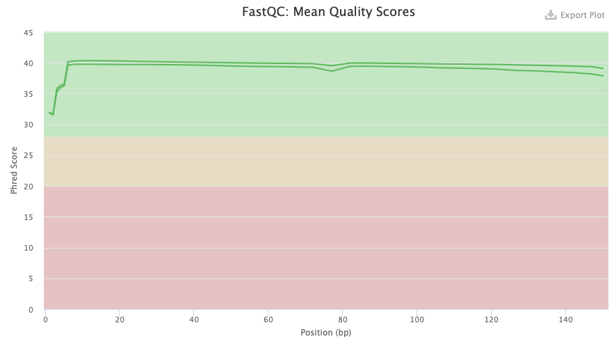
Figure 1. FastQC quality check result from Illumina DNA data.
PacBio DNA:
In figure 2 for PacBio DNA instead, the phred score is in the red area all the way through. This can be due to that PacBio has a higher error rate than Illumina. Which also is why we will later use Illumina to correct the assembly from the PacBio data.
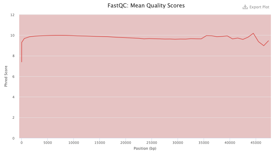
Figure 2. FastQC quality check result from PacBio DNA data.
Illumina Transcriptome
Comparing figure 3 and 4 of Illumina for the transcriptome we can see the two cases of untrimmed and trimmed reads. In the trimmed case there are four lines instead of two as for the untrimmed ones. This is due to that the trimming results in both paired and unpaired reads, forward and reverse for each. The two upper lines of the trimmed one are in a similar score as for the untrimmed ones. But the others are of a bit lower quality. It is expected that the quality will be about the same as the trimming removes adapters for example, which should not affect the score so much.
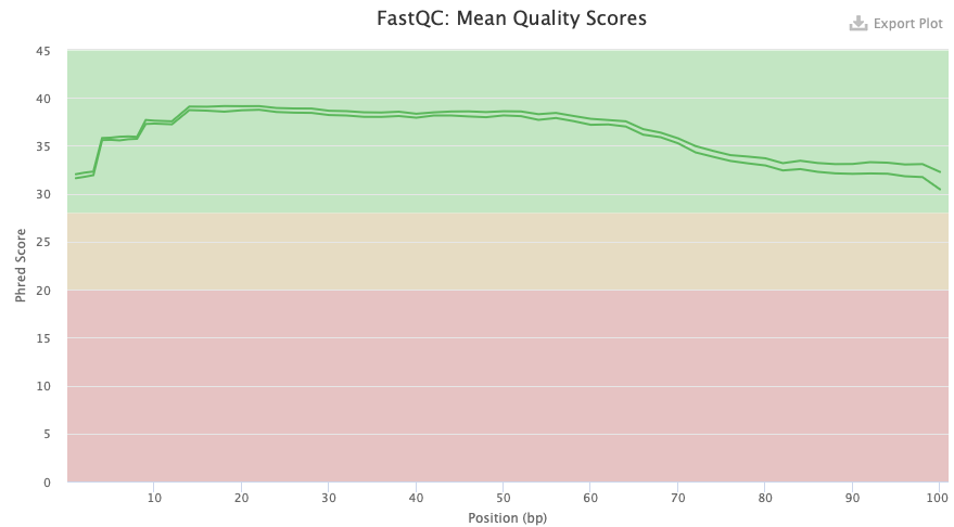
Figure 3. FastQC quality check result from Illumina transcriptome data untrimmed.
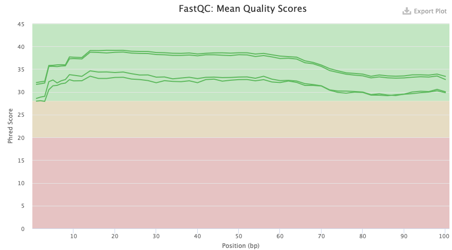
Figure 4. FastQC quality check result from Illumina transcriptome data trimmed.
In figure 5 the per sequence GC content for all samples can be seen. In the plot for Illumina DNA there is roughly only one peak, which is good. While instead looking at the transcriptome plots the double peaks indicates that there can be contamination in the sample. There is a tendency to double peaks in the PacBio DNA also. What also can be notised for the transcriptomes is that the GC content is higher than the others. A high GC content can cause a less good assembly if that would have been done on these reads, also the duplication levels are higher for the transcripts which also can be problematic.
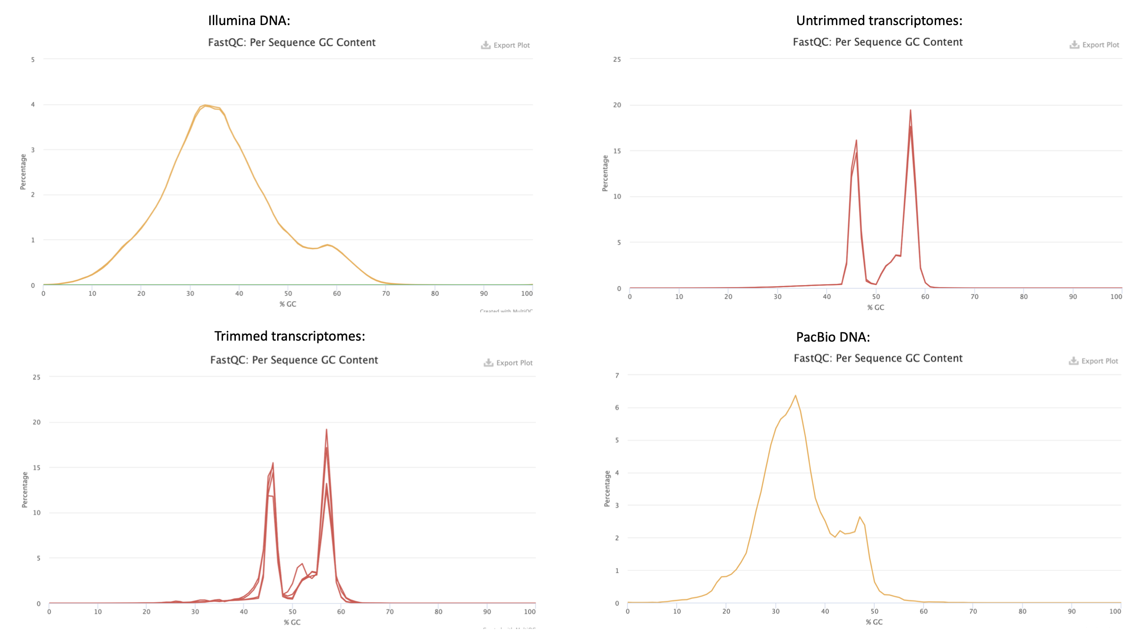
Figure 5. Per sequence GC content from FastQC quality check result from all the analysed samples.
All the per sequence quality score in figure 6 show a quite clear peak to the right in the figure, which is a somewhat expected good result.
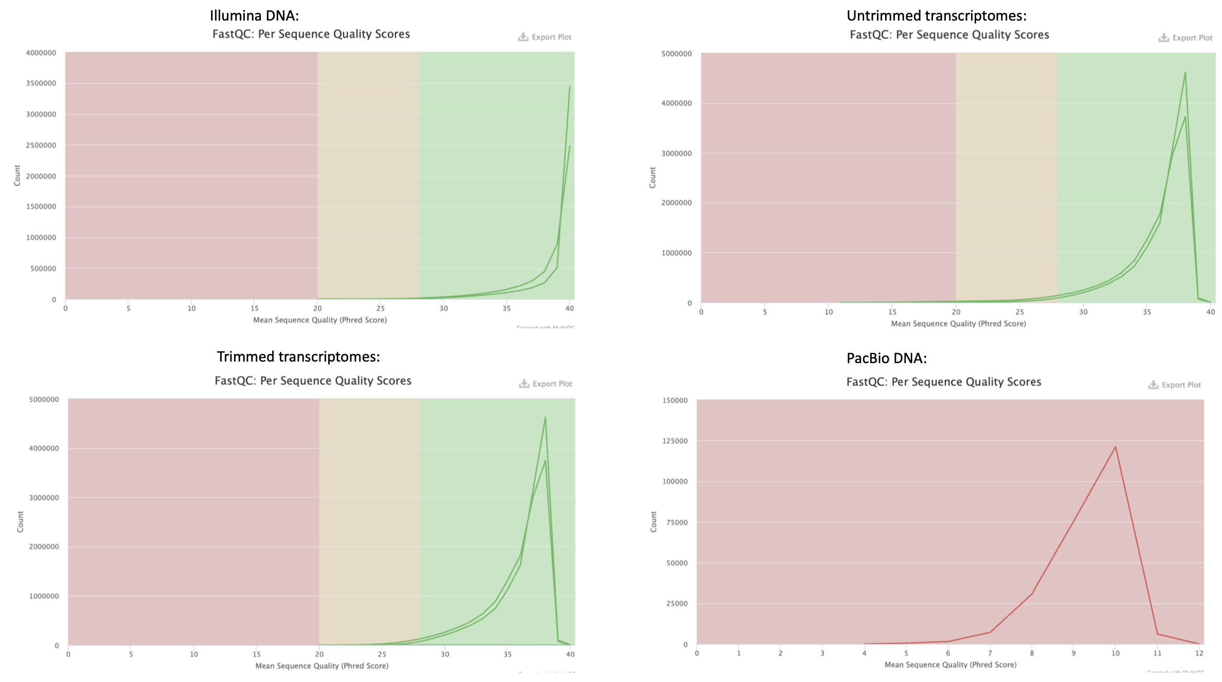
Figure 6. Per sequence quality score from FastQC quality check result from all the analysed samples.
The Genome Assembly of the scaffold with PacBio DNA reads were run with the bash script named Genome_assembly_PacBio.sh. This script uses the software Canu to do the assembly, were the genome size were specified to 24 m as a parameter.
By creating an index with the resulting file from the assembly, the mapping were performed with the software BWA to map the assembled PacBio DNA reads with the Illumina DNA reads. The purpose with this was to in the next step use the Illumina reads to increase the quality of the assembly by correcting misstakes as PacBio has a quite high error rate. The script used is called Mapping_Illumina_PacBio.sh. The resulting files were also converted to bam format instead of sam format for further analysis. These lastly mentioned steps were done using the software samtools with the tools sort and index. These commands can also be seen in the script.
The software Pilon is used to correct the assembly with the purpose previously described. The script for doing this is named Correct_assembly_DNA.sh. The correction is performed by using the mapped PacBio and Illumina DNA reads along with the assembly.
By using the software Quast the corrected assembly were evaluated. The script for performing this is named Assembly_evaluation_DNA.sh.
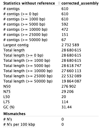
Figure 7. Statistics from the report of the assembly evaluation.
In figure 7 the statistics from the report of the assembly evaluation can be seen. These values can be compared to values from a reference genome of the same scaffold used here (scaffold 10). A high N50 value is good, as well as the number of contigs preferably should be as few as possible. The genome size of the assembly should also be as close as possible to the actual genome size, which in the article is estimated to be 800 Mb, but since we are only analysing one scaffold that comparison it not applicable for this analysis.
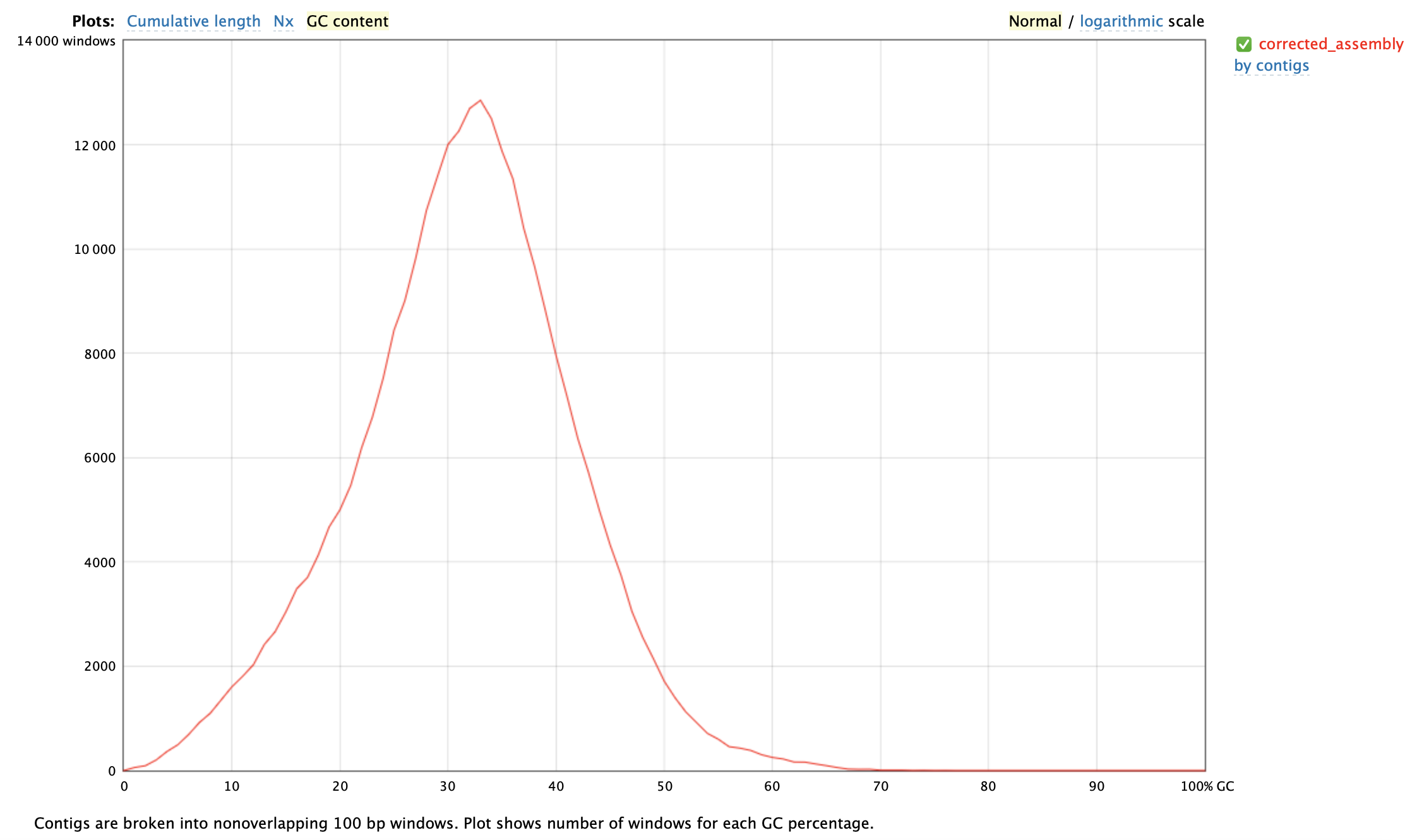
Figure 8. Plot of GC content from the assembly evaluation.
In figure 8 the GC content can be seen from the assembly evaluation. In the figure there is only one peak, which is somewhat a normal distribution, which is an indication that there are no contamination and that is looks good.
The RepeatMasker software were used for removing repeated regions in the corrected assembly. The parameters used were default except for the species, which were selected to be Malvaceae with taxonomy number 3629 (the family of Durian fruit) which was found on NCBI taxonomy browser. The software were run with the script Remove_repeats_DNA.sh.
Using the script Mapping_DNA_transcriptome.sh the software star were run to map the transcriptome (RNA) with the DNA were repeats had been removed. Firstly, an index were created with the corrected assembly as input. Then star were run one time for each pair of forward and reverse transcriptome file, with an "&" sign after each command to specify that the runs should be performed in parallel to speed it up. A flag was used to specify that the output format should be unsorted BAM file since that was needed for further analysis. The flag readFilesCommand was also used as the input files are zipped.
Firstly all required modules were loaded. Then the augustus configuration file were copied to enable access to it, this were done with the following command when standing in this folder:
/home/ellens/Durian_fruit/Analyses/12_Structural_annotation/
source $AUGUSTUS_CONFIG_COPY
Then another command were used to get writing permission to the augustus configuration file. This can be seen below:
chmod a+w -R /home/ellens/Durian_fruit/Analyses/12_Structural_annotation/augustus_config/species/
To copy the GeneMark key this following command were used:
cp -vf /sw/bioinfo/GeneMark/4.33-es/snowy/gm_key $HOME/.gm_key
These commands can also be seen out commented in the script with the braker command in the file Structural_annotation.sh. Since the RepeatMasker were used with hard masking (replacing letters in repetitive regions with N), there were no flag inserted for this (which should have been done for soft masked data). A flag used were --gff3 to get the output in gff3 format which were needed for the differential expression analysis with HTSeq. The specie were also specified with a flag as "Durio zibethinus". As input to braker the corrected assembly and the ten mapped DNA/transcriptome files were used. The output from this analysis were among others a file named augustus.hints.gff3.
The result from this structural annotation were used for the differential expression in the software HTSeq.
To do a functional annotation the software eggNOGmapper were used, which were run with the script Functional_analysis.sh. The corrected assembly were used as input to eggNOGmapper. In this software several options are possible, for this analysis diamond blastp were used, which is also the default. In the command a flag was used to specify the type of sequence the input data is, this one was set to "genome". The result from the functional analysis were used to see a suggested function for an interesting gene, more about that further in the analysis description.
The software HTSeq were used to count the mapping reads to genomic features. To use this, the bam files from the mapping of DNA and transcriptome were sorted, this were performed with the script Sort_BAM_files.sh. After that the script Read_counting.sh were run to use HTSeq were the agusutus.hints.gff file from the structural annotation were used along with each of the sorted files as input. Flags are used to specify that the mapped files are sorted by position, which one is the ID attribute as well as that the input format is in BAM. The output are one file for each mapped file that specify the counting. These are downloaded to the local computer with Rsync to be used in R with the package DESeq2.
DESeq2 is a package used in R with RStudio. It is installed using this command:
if (!require("BiocManager", quietly = TRUE))
    install.packages("BiocManager")
BiocManager::install("DESeq2")
The code for doing the analysis can be found in the file DeSeq2.R. Using DESeq2 a heat map and a PCA are performed with the read counting as input, the results can be seen below.
Heat map
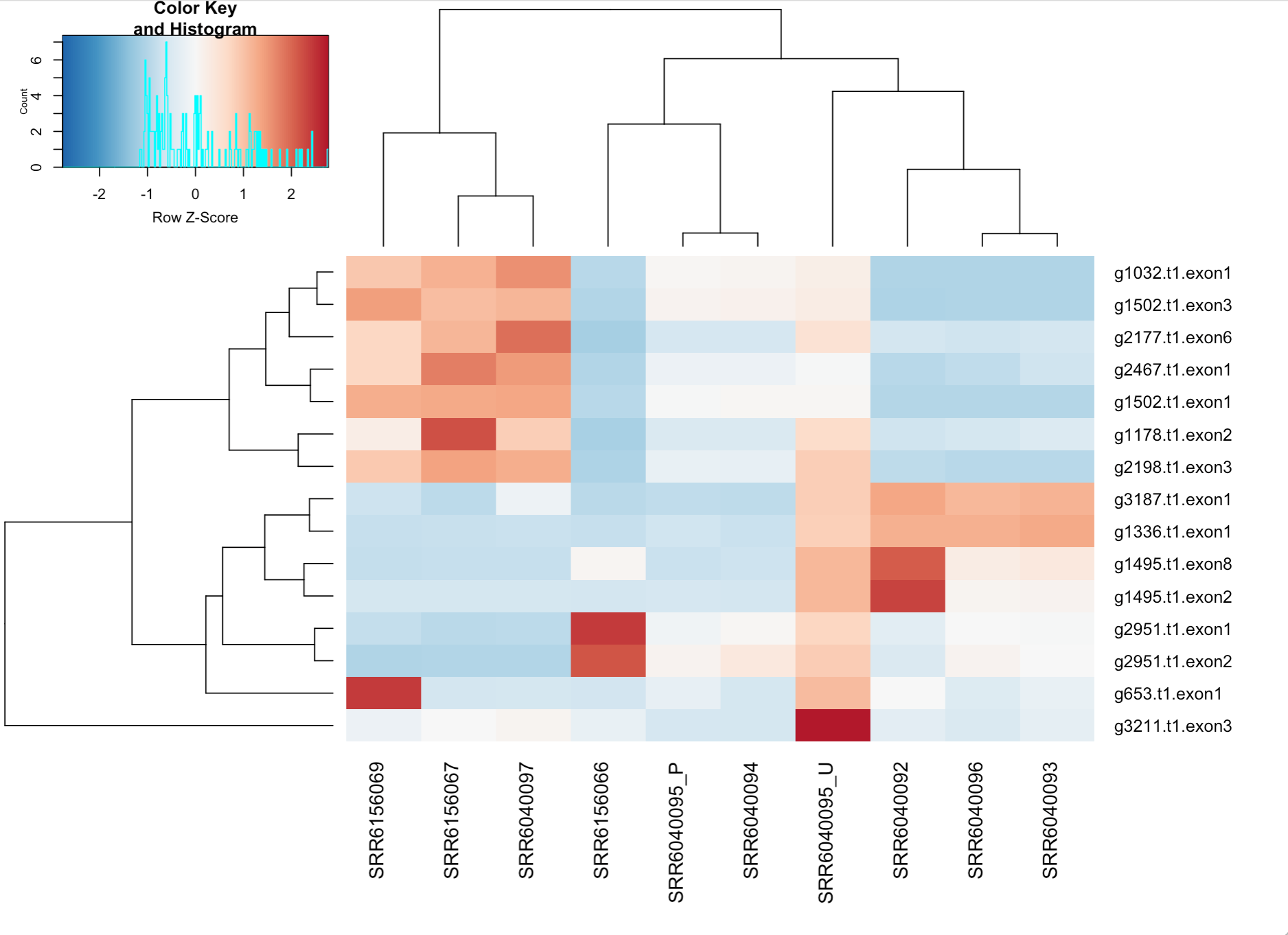
Figure 9. Heat map from the read counting, showing the 15 genes with most variance.
In figure 9 the heat map can be seen. On the y-axis there are the 15 genes with the most variance. Each of these are picked out and searched for in the augustus.hints.gff3 file which were produced from the structural annotation analysis step. There, another name in the format "tig00000XXX_pilon" is noted which in its turn is searched for in the functional annotation output file Functional_annotations.emapper.gff. If a hit was found with the correct start position, the annotated function of this hit was noted. This resulted in two hits of the 15 checked genes. These can be seen below in table 1.
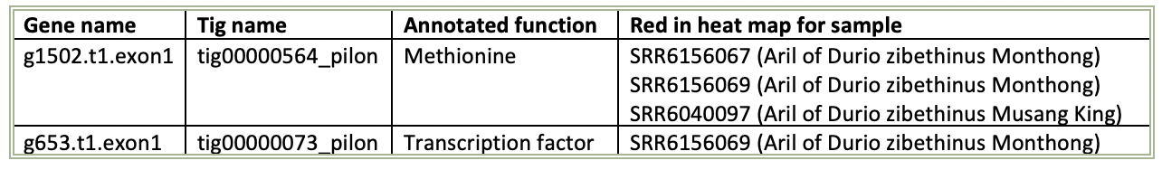
Table 1. Table with the genes of interest and their annotated function.
The gene g1502 were red in the heat map for the three specified samples in table 1, but only light red which means that there are not as much expression variance compared to the other samples compared to if it would have been dark red. The color scale between red and blue is an indication of how much the gene expression varies. The second gene in table 1 is g653 which is dark red for the specified sample from aril in the Monthong. This means that the variation of expression is larger between the samples for this gene.
PCA
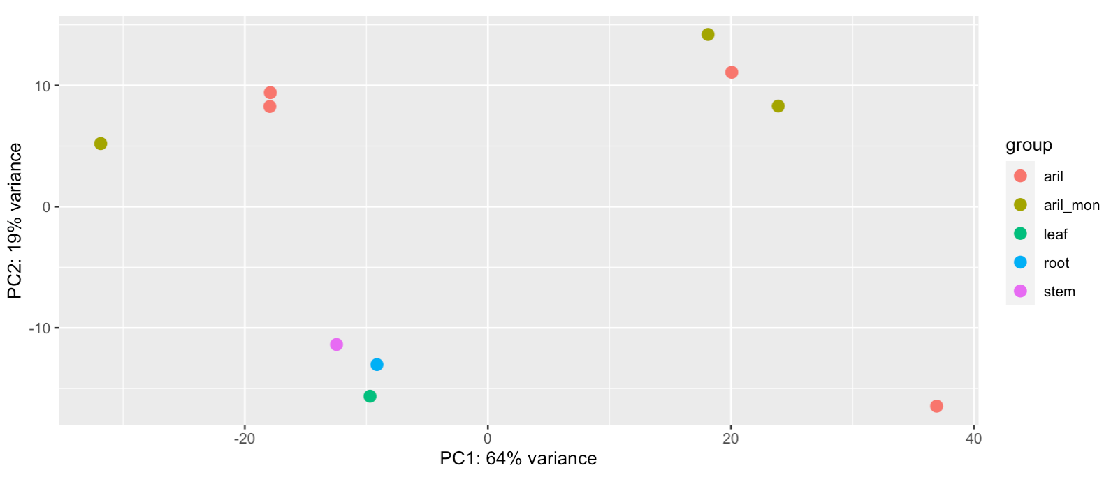
Figure 10. PCA from the read counting.
In figure 10 of the PCA there can be seen that the sample from stem, root and leaf are close to each other. That means that the variance of expression between these are quite low. While for the samples of aril of Musang King and the samples from aril of Monthong, the data points are more far away from each others. This means that there are more variance in expression between these samples, and that is therefore an indication that there are differences in how genes are expressed in the arils between different fruits.